7 Creating a script
Now that we have a bunch of fundamental skills, we are going to integrate them from top-to-bottom in the form of a brand new script. This will help us practice what it actually feels like to explore and analyze a data set on our own.
- Each saved script must be able to be run sequentially from top to bottom without failing.
source()function or the Source button should run without error.- The document should proceed in a rational order.
7.1 Pseudo-script form
# ------------------------------------------------------------------------------
# Title: The general form template of a script
# Date
# Author
# ------------------------------------------------------------------------------

# Load libraries
require(tidyverse)

# Load data
df <- read_csv("file.csv")

# Analyze data
df %>%
  group_by(groups) %>%
  summarise(avg = mean(dep_var))

# Visualize
df %>%
  ggplot() +
  geom_boxplot(aes(x = ind_var, y = dep_var))

# Statistics
mod <- aov(dep_var ~ ind_var, data = df)
This is just an example of a general structure of the script. When you are actually exploring your data, you should have more exploration, analysis, and visualization in your script.
7.2 Script for CTmax data
# CT max data ------------------------------------------------------------------
# Thomas O'Leary

# Load library
library(tidyverse)

# Load data
df <- read_delim("Populations_CTmax.csv", delim = ";")
# Rows: 336 Columns: 3
# ── Column specification ────────────────────────────────────────────────────────
# Delimiter: ";"
# chr (2): Population, Treatment
# dbl (1): CTmax
#
# ℹ Use `spec()` to retrieve the full column specification for this data.
# ℹ Specify the column types or set `show_col_types = FALSE` to quiet this message.

# Get averages and standard deviations
df %>%
  group_by(Population, Treatment) %>%
  summarise(ct_max = mean(CTmax),
            sd = sd(CTmax))
# `summarise()` has grouped output by 'Population'. You can override using the
# `.groups` argument.
# # A tibble: 14 × 4
# # Groups:   Population [7]
#    Population Treatment ct_max    sd
#    <chr>      <chr>      <dbl> <dbl>
#  1 Chorges    Control     37.7 0.373
#  2 Chorges    Hardening   38.3 0.460
#  3 Frankfurt  Control     37.9 0.515
#  4 Frankfurt  Hardening   38.5 0.458
#  5 Hamburg    Control     37.3 1.10
#  6 Hamburg    Hardening   38.1 0.301
#  7 Hannover   Control     37.6 0.948
#  8 Hannover   Hardening   38.3 0.372
#  9 Mols       Control     37.1 0.395
# 10 Mols       Hardening   38.1 0.316
# 11 Siena      Control     38.1 0.349
# 12 Siena      Hardening   38.7 0.391
# 13 Skagen     Control     36.8 0.517
# 14 Skagen     Hardening   37.8 0.408

# Make plots ----

# Make a box plot
df %>%
  ggplot() +
  geom_boxplot(aes(x = Treatment,
                   y = CTmax)) +
  theme_classic()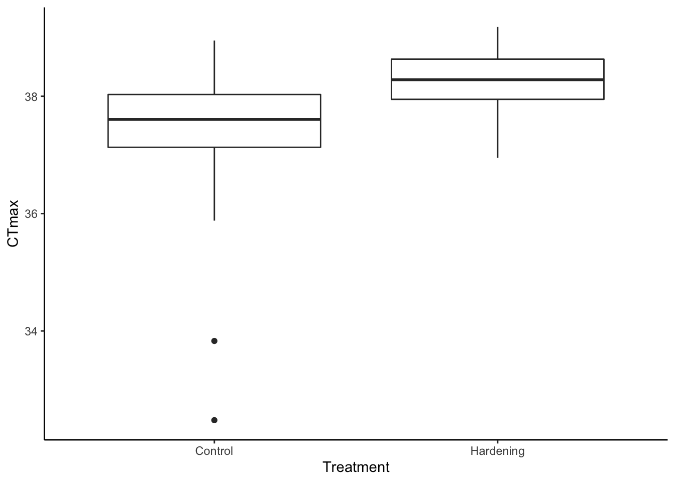
# Color by population
df %>%
  ggplot() +
  geom_boxplot(aes(x = Treatment,
                   y = CTmax,
                   color = Population)) +
  theme_classic()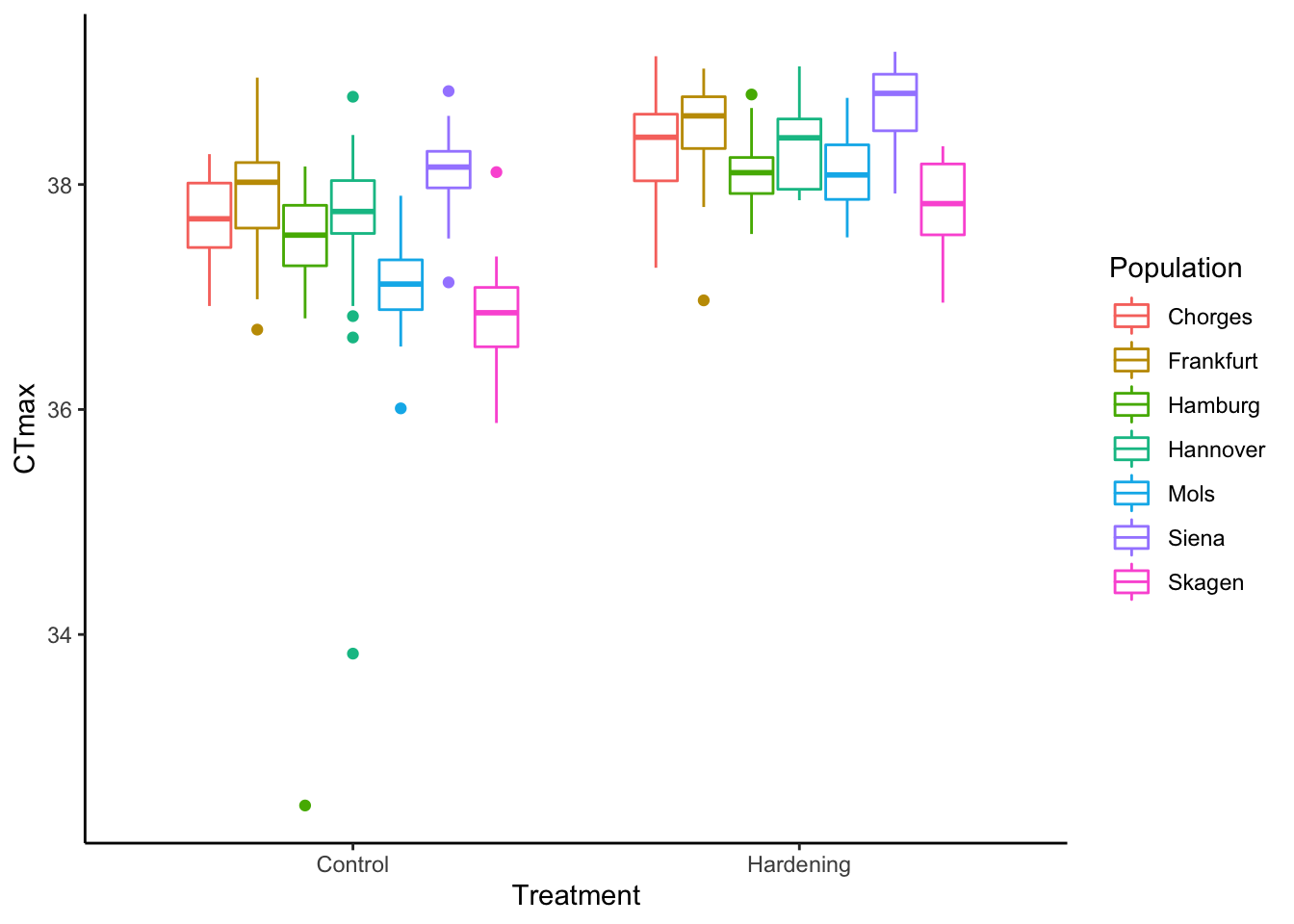
# Run analysis
mod <- aov(CTmax ~ Population*Treatment,
           data = df)

broom::tidy(mod)
# # A tibble: 4 × 6
#   term                    df sumsq meansq statistic   p.value
#   <chr>                <dbl> <dbl>  <dbl>     <dbl>     <dbl>
# 1 Population               6 40.1   6.68      22.7   2.75e-22
# 2 Treatment                1 48.9  48.9      166.    6.99e-31
# 3 Population:Treatment     6  2.63  0.439      1.49  1.82e- 1
# 4 Residuals              322 94.9   0.295     NA    NA