2 First principles
There are many languages in which you can program (e.g. python, java, C++), but here we are going to use R.
2.1 R & RStudio
R is primarily used for statistical programming and data visualization. It comes with a minimal R terminal – which is just a place that allows you to execute the code. However, we are going to use RStudio as our integrated development environment (IDE).
If coding is like painting, then you can think of R as the raw materials – primary paint colors and a few paint brushes; painting would be impossible without these basic tools. However, RStudio – aptly named – is like a painting studio. It is not necessary to the task of painting, but it is immensely helpful. In this studio, you will find a drafting table, canvas, easel, and a palette. And finally at risk of extending this metaphor to its breaking point – there is also a world of skilled painters who have developed specialized sets of paint brushes and other tools. And they have made them available to you for free. These are called packages. We will get into this later!
2.2 Let’s start coding
Step 1: Open RStudio and get a lay of the land.
RStudio has four main panels: (i) source, (ii) console (iii) environment & history, (iv) files, plots, packages, & help information.
- The source panel is where you will create and save your code.
- The console actually executes the code.
- The environment shows objects that you have assigned or added to your working space. History shows previously executed code.
- Files shows the directories (i.e. folders) on your computer. Plots is where your plots will be visualized. Packages and Help tabs give you useful documentation related to packages and functions, etc.
I like to use RStudio projects to store my data, scripts, results, and figures. This helps keep a good directory structure3 – example below – so that everything related to the project is in the same place in an orderly fashion.
Save your files with useful names in an ordered nested directory structure. -
project_name/scripts/load_clean_data.R-project_name/scripts/analyze_data.R-project_name/data/raw_data.csv-project_name/figures/fig_1.pdf
It is a good idea to avoid using the
.RDatafile that comes with your project to save the objects in your working environment. You want your self-contained script to you can change that in your RStudio settings like so. This section of does a good job of explaining why this is good practice.
Step 2: Create a new R script!
It is good practice to include useful information at the top of the script. This will help both your future-self and a potential collaborator recognize quickly what the script is all about. An example is below:
# ------------------------------------------------------------------------------
# REU Data Science Workshop Summer 2022 -- Learning some R basics today
# June 13, 2022
# TS O'Leary
# ------------------------------------------------------------------------------

# Comments are useful throughout the document
# The #-symbol indicates that the following is merely text and
#    R will not interpret it as code

# I am getting a little a head of myself -- but below is math.
3 + 3 # You can comment on the right of executable code, but I think it's ugly.
# [1] 6
Now that we have a script open, we will begin learning some R 😄.
Step 3: Code…
2.3 Basic math
# Try adding
2 + 3
# [1] 5

# Or multiplying
2 * 3
# [1] 6

# Or something more complicated
(2 * 3)^2
# [1] 36
This is great, but it just makes R seem like a really fancy calculator. The real utility of R comes from the fact that you can create scripts, objects, and functions to reproducibly analyze your data.
2.4 Creating objects
In R, you can create variables (or objects) which are place-holders for some value that may change. These variables are assigned with the <- operator. For example, if you had two variables x & y, you could assign their respective values together with the following code:
# Assign values to variables
x <- 2
y <- 3
Then, you can perform some math on them:
# Add together values
x + y
# [1] 5
Quick note on the alternative
=operator. It is possible to assign values to objects using the equal sign (e.g.x = 2). But I think it is best to avoid this notation for reasons that are best explained later. But at risk of overexplaining I will say now that using<-avoids confusion with the==function which accesses equality. It also reserves the equal sign for the assignment of argument values within a function. Additionally, I think the<-operator is a better visualization of what the operator is actually doing (i.e. in the case ofx <- 2you are assigning the integer2to the variablex). If that doesn’t make any sense, that’s okay. We’ll get to that stuff later.
2.4.1 Naming objects
It is good practice to be careful and deliberate when you are naming variables within your code. You want the variables to be both short – so they are easy to type and read – and also descriptive – so you remember what they represent.
You are allowed to use letters, numbers, and underscores (_) in variable naming.
# Set variable values
greet <- "Hello"
name <- "Tom"
greetandnameare both descriptive and short variable names for the values that they represent.
Then you can print them out together like this:
# Print both variables
print(c(greet, name))
# [1] "Hello" "Tom"
Or even paste it together to make a sentence:
# Paste together
paste(greet, name, ", nice to meet you")
# [1] "Hello Tom , nice to meet you"
Quick challenge: Find a way to get rid of that pesky space before the comma.
2.4.1.1 The snake & camel
There are two “cases” that are widely used in naming things in programming.
snake_case– which uses underscores (_) between words.- This is my preferred case.
camelCase– which starts with a lower case and each subsequent word begins with a capital letter.
chaoscasevariablenaming– You can name things without marking the separation between words. But this method obviously stinks.
2.4.1.2 Forbidden characters
_underscore at the beginning of the variable name- e.g.
_variable_name
- e.g.
- a number at the beginning
- e.g.
1_variable
- e.g.
2.4.1.3 Characters to avoid
.– dots (or periods) are allowed, but it is better to reserve the dot for other stuff.
Final Note: I like to make my function names with verbs. A function performs a specific action, so you can make that clear with a descriptive verb.
2.5 Data types
There are a several fundamental data types in R and it is worthwhile taking a moment to distinguish them.
- Atomic vectors are one-dimensional array of a single object type.
- Lists are a one-dimensional group of different object types.
- A matrix is a two-dimensional array of a single object type.
- A data frame is a two dimensional grouping of different object types.
The relationship of these terms to each other is summarized in the table below.
| Dimensions | Homogenous | Heterogeneous |
|---|---|---|
| 1-D | atomic vector | list |
| 2-D | matrix | data frame |
If it seems abstract now, don’t fret, we will talk about each of these data types in detail now.
2.5.1 Object class
- character strings
- numeric
- integers
- double
- logical
- factor
- vector of lists
# Character
char <- "letters or anything -- 1 $ % !"
char
# [1] "letters or anything -- 1 $ % !"

# Check the class
# class() is a function in base R that checks the class of an object
?class() # the question mark asks RStudio to give you the Help info on that function
class(char)
# [1] "character"
# Numeric
num <- 1
num
# [1] 1
class(num)
# [1] "numeric"# Logical
log <- FALSE
log
# [1] FALSE
class(log)
# [1] "logical"We just stumbled into another no-no for variable naming. It is bad practice to use variable names that are also functions.
log()is actually the natural logarithm function. Thelog()function will still work – even withlogbeing an object saved as FALSE in the environment – but it gets messy.
# log() is actually the natural logarithm function
?log
log(exp(1))
# [1] 1
Note:
TRUE&FALSEcan also be written short hand asTorF. But it is more clear to use the full word. Typing a few more characters will not kill you.
# Factor
fac <- as.factor("cats")
fac
# [1] cats
# Levels: cats
class(fac)
# [1] "factor"
Notice how
fachasLevels: catswhich indicates that there is one level to the factor named cats. If this is confusing we will get to factors in more detail once we
2.5.2 Vectors & Indexing
2.5.2.1 Concatenate c() function
The c() function combines arguments to form a vector.
For example:
# Set x as a numerical vector
vec <- c(1, 4, 2, 7)

vec
# [1] 1 4 2 7
You can use other base functions to explore the properties of the object x.
# Determine the class of vec
class(vec)
# [1] "numeric"

# Print out the length of vec
length(vec)
# [1] 4

# Summary statistics of vec
summary(vec)
#    Min. 1st Qu.  Median    Mean 3rd Qu.    Max.
#    1.00    1.75    3.00    3.50    4.75    7.00
2.5.3 Indexing
Indexing is just a fancy way of saying that you are accessing specific parts of a larger object.
For example:
# Indexing the atomic vector vec at the first position
vec[1]
# [1] 1
It is worth noting that in R, indexing begins at
1. For those of you unfamiliar with programing in another language that may seem like a ridicuolous thing to say, but most languagues (e.g. python, MatLab) begin indexing at0.
You can index multiple objects at once:
# Indexing the atomic vector vec at the second and third position
vec[c(2, 3)]
# [1] 4 2
Or you can index based on a logical statement
# Vector where the values are greater than 3
vec[vec > 3]
# [1] 4 7

# Vector where the values are equal to 7
vec[vec == 7]
# [1] 7

# There are also functions designed to do this
subset(vec, vec == 7)
# [1] 7
R also has cool short hand ways to create sequences.
# The : operator sequences a vector by 1 from the left to the right side
1:16
#  [1]  1  2  3  4  5  6  7  8  9 10 11 12 13 14 15 16

16:1 # Produces the decreasing sequence
#  [1] 16 15 14 13 12 11 10  9  8  7  6  5  4  3  2  1

# What if you want to exclude a number?
c(1:4, 6:16)
#  [1]  1  2  3  4  6  7  8  9 10 11 12 13 14 15 16

# Check out the seq function with ?seq and then use it
seq(from = 1, to = 16, by = 1)
#  [1]  1  2  3  4  5  6  7  8  9 10 11 12 13 14 15 16
seq(from = 1, to = 16, by = 2)
# [1]  1  3  5  7  9 11 13 15
seq(from = 1, by = 1, length.out = 16)
#  [1]  1  2  3  4  5  6  7  8  9 10 11 12 13 14 15 16
2.5.4 Accessing equality
Now we have two vectors x and y – let’s say we want to know what if any differences there are between the two vectors. There are several ways that you could do that
I have created two vectors x and y. In y, there is one missing number from one to thirty, but we don’t know which. This is how you could find out with code.
# Print the vectors
x
#  [1] 19  7 21 24 11  1 23 25 20 10  9  5 14 30  2 13  3 29 28  8  4  6 15 26 27
# [26] 17 12 18 16 22
y
#  [1] 27 30  2 15 14 11 12 13 26  4 29 23  6 21 16 18 20 25  1  3 22 28  5 10  9
# [26] 24 17 19  8

# We know that they have different lengths
length(x)
# [1] 30
length(y)
# [1] 29

# We could check one-by-one through indexing
x[1] == y[1]
# [1] FALSE
x[1] == y[2] # But that would be a nightmare...
# [1] FALSE

# The %in% operator returns a logical vector that accesses whether each value
#   of x is present in y
x %in% y
#  [1]  TRUE FALSE  TRUE  TRUE  TRUE  TRUE  TRUE  TRUE  TRUE  TRUE  TRUE  TRUE
# [13]  TRUE  TRUE  TRUE  TRUE  TRUE  TRUE  TRUE  TRUE  TRUE  TRUE  TRUE  TRUE
# [25]  TRUE  TRUE  TRUE  TRUE  TRUE  TRUE

# Similarly adding the ! operator returns a logical vector that accesses
#   each value of x that is not present in y
!(x %in% y)
#  [1] FALSE  TRUE FALSE FALSE FALSE FALSE FALSE FALSE FALSE FALSE FALSE FALSE
# [13] FALSE FALSE FALSE FALSE FALSE FALSE FALSE FALSE FALSE FALSE FALSE FALSE
# [25] FALSE FALSE FALSE FALSE FALSE FALSE

# The which function gives the indices for which the logical vector is TRUE
which(!(x %in% y))
# [1] 2

# To figure out the value of x that is at position where the above logical is T
x[which(!(x %in% y))]
# [1] 7
2.6 Data frames
Most often I find that when I am working with data that I collected or generated, I am working with data frames – which are tables. Data frames can contain different object classes (e.g. numeric, character, factor) and are useful for storing data that has multiple pieces of information associated with each observation.
For the most part, those will be loaded into the environment in R from a text file (e.g. comma separated values, csv) with a function call like read_csv("path/to/file.csv"). We will talk about this in more detail later. But for now, we are going to make our own data frame and then play with some built in data.
2.6.1 Creating a data frame
# Create vectors
sample_id <- paste("sample", 1:16, sep = "_")
x <- 1:16
sqrt_x <- sqrt(x)

# Merge together in a data frame
df <- data.frame(sample_id = sample_id,
                 x = x,
                 sqrt_x = sqrt_x)

df
#    sample_id  x   sqrt_x
# 1   sample_1  1 1.000000
# 2   sample_2  2 1.414214
# 3   sample_3  3 1.732051
# 4   sample_4  4 2.000000
# 5   sample_5  5 2.236068
# 6   sample_6  6 2.449490
# 7   sample_7  7 2.645751
# 8   sample_8  8 2.828427
# 9   sample_9  9 3.000000
# 10 sample_10 10 3.162278
# 11 sample_11 11 3.316625
# 12 sample_12 12 3.464102
# 13 sample_13 13 3.605551
# 14 sample_14 14 3.741657
# 15 sample_15 15 3.872983
# 16 sample_16 16 4.000000

class(df)
# [1] "data.frame"
The $ operator allows you to extract a specific column from a data frame. For example,
# Returns the x column in a numeric vector
df$x
#  [1]  1  2  3  4  5  6  7  8  9 10 11 12 13 14 15 16
If you want to add a new column with a new_vector, you can assign to a new_col_name with the <- operator, according to the following form df$new_col_name <- new_vector. For example,
# Adding a column, x_2, with x-squared
df$x_2 <- df$x^2

# Adding a column, y, with 8.5 subtracted from x
df$y <- df$x - 8.5

df
#    sample_id  x   sqrt_x x_2    y
# 1   sample_1  1 1.000000   1 -7.5
# 2   sample_2  2 1.414214   4 -6.5
# 3   sample_3  3 1.732051   9 -5.5
# 4   sample_4  4 2.000000  16 -4.5
# 5   sample_5  5 2.236068  25 -3.5
# 6   sample_6  6 2.449490  36 -2.5
# 7   sample_7  7 2.645751  49 -1.5
# 8   sample_8  8 2.828427  64 -0.5
# 9   sample_9  9 3.000000  81  0.5
# 10 sample_10 10 3.162278 100  1.5
# 11 sample_11 11 3.316625 121  2.5
# 12 sample_12 12 3.464102 144  3.5
# 13 sample_13 13 3.605551 169  4.5
# 14 sample_14 14 3.741657 196  5.5
# 15 sample_15 15 3.872983 225  6.5
# 16 sample_16 16 4.000000 256  7.5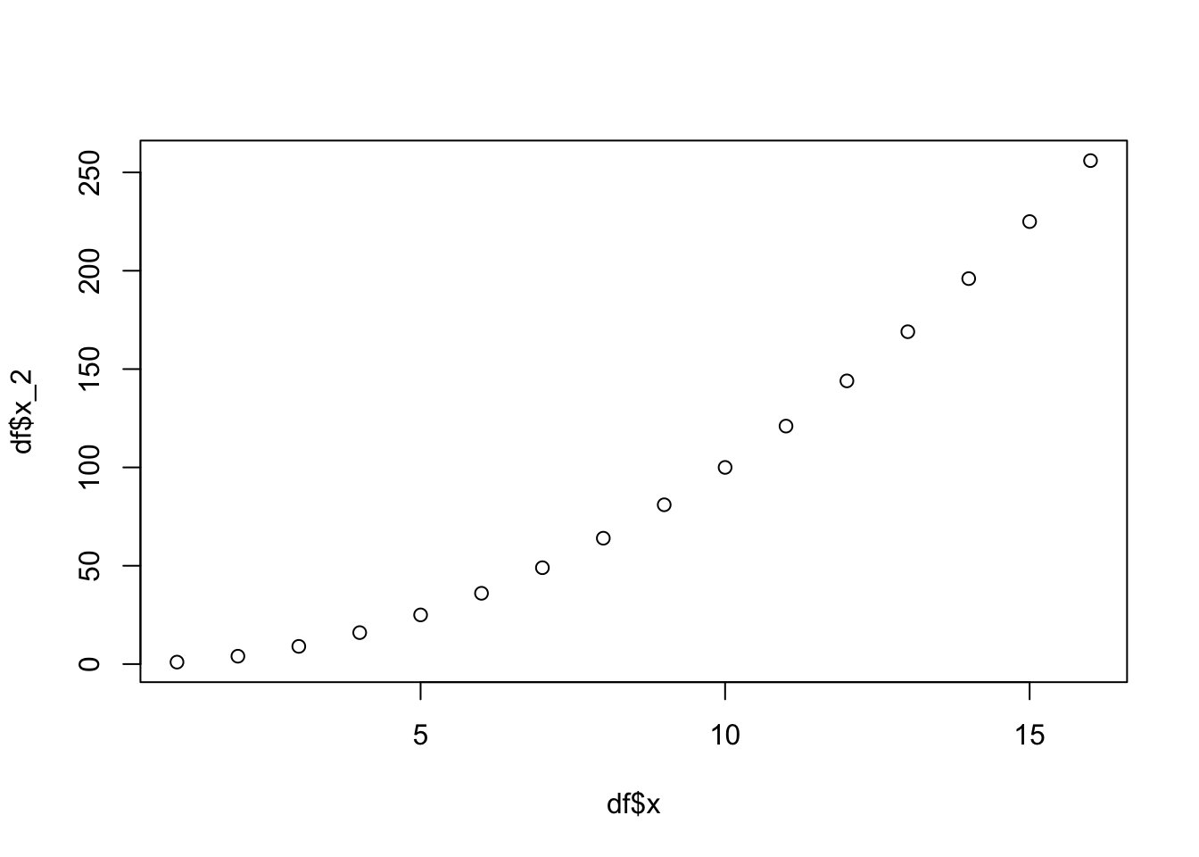
Obviously, the project itself does not create this orderly directory structure, but it just fosters the environment where you can build a good directory structure.↩︎