Alex
# ------------------------------------------------------------------------------
# Alex's Survival Data Analysis with Workshop
# Alex Lewis
#----------------------------------------------------------------------------
#Load Libraries
require(tidyverse)
require(drc)
# Loading required package: drc
# Loading required package: MASS
#
# Attaching package: 'MASS'
# The following object is masked from 'package:dplyr':
#
# select
#
# 'drc' has been loaded.
# Please cite R and 'drc' if used for a publication,
# for references type 'citation()' and 'citation('drc')'.
#
# Attaching package: 'drc'
# The following objects are masked from 'package:stats':
#
# gaussian, getInitial
# Load data
surv <- read_csv(here::here("student_data/raw_survival_alex_25JUL2022.csv"))
# Rows: 101 Columns: 6
# ── Column specification ────────────────────────────────────────────────────────
# Delimiter: ","
# chr (2): Genotype, Shock_Date
# dbl (4): Temperature, Eggs, Hatched_24, Hatched_48
#
# ℹ Use `spec()` to retrieve the full column specification for this data.
# ℹ Specify the column types or set `show_col_types = FALSE` to quiet this message.
lock_surv <- read_delim(here::here("student_data/raw_survival_lockwood_et_al_2018.txt"),
delim = "\t") %>%
dplyr::rename(Genotype = genotype,
Eggs = eggs,
Hatched_48 = hatched,
Temperature = temperature)
# Rows: 933 Columns: 6
# ── Column specification ────────────────────────────────────────────────────────
# Delimiter: "\t"
# chr (2): genotype, region
# dbl (4): temperature, eggs, hatched, survival
#
# ℹ Use `spec()` to retrieve the full column specification for this data.
# ℹ Specify the column types or set `show_col_types = FALSE` to quiet this message.
# Combine data
surv <- bind_rows(surv, lock_surv)
# LT50-----------------------------------------------------------------------
lt_surv_curv <- surv %>%
filter(!str_detect(Genotype, "Canton")) %>%
group_by(Genotype) %>%
nest() %>%
mutate(fit = map(data, ~ drm(Hatched_48/Eggs ~ Temperature,
data = .x,
weight = Eggs,
fct = LL.3(names = c("slope",
"upper limit",
"LT50")),
type = "binomial")),
lt_s = map(fit, ~ ED(.x,
c(10, 50, 90),
interval = "delta",
display = FALSE))) %>%
mutate(tidy_fit = map(fit, broom::tidy)) %>%
mutate(lt_10 = lt_s[[1]][[1]],
lt_50 = lt_s[[1]][[2]],
lt_90 = lt_s[[1]][[3]])
# Calcu.ate mean and sd from locale groups
lt_surv_curv %>%
filter(!str_detect(Genotype, "X")) %>%
mutate(locale = case_when(str_detect(Genotype, "FLCK") ~ "Florida",
str_detect(Genotype, "VT") |
str_detect(Genotype, "BEA") |
str_detect(Genotype, "RFM") ~ "Temperate",
str_detect(Genotype, "JP") ~ "Japan",
str_detect(Genotype, "FR") ~ "France",
TRUE ~ "Tropical")) %>%
group_by(locale) %>%
summarise(lt50_mean = mean(lt_50),
lt50_sd = sd(lt_50),
count = n()) %>%
mutate(lt50_se = lt50_sd/sqrt(count),
lt50_95ci = lt50_se*1.96)
# # A tibble: 5 × 6
# locale lt50_mean lt50_sd count lt50_se lt50_95ci
# <chr> <dbl> <dbl> <int> <dbl> <dbl>
# 1 Florida 34.9 0.268 6 0.109 0.214
# 2 France 35.0 0.511 2 0.361 0.708
# 3 Japan 34.4 0.387 2 0.274 0.537
# 4 Temperate 34.9 0.449 19 0.103 0.202
# 5 Tropical 35.9 0.414 5 0.185 0.363
lt_surv_curv
# # A tibble: 36 × 8
# # Groups: Genotype [36]
# Genotype data fit lt_s tidy_fit lt_10 lt_50 lt_90
# <chr> <list> <list> <list> <list> <dbl> <dbl> <dbl>
# 1 FLCK 02 <tibble [8 × 7]> <drc> <dbl [3 × 4]> <tibble> 33.6 34.9 36.2
# 2 FLCK 03 <tibble [8 × 7]> <drc> <dbl [3 × 4]> <tibble> 33.4 34.5 35.7
# 3 FLCK 05 <tibble [8 × 7]> <drc> <dbl [3 × 4]> <tibble> 33.7 34.7 35.7
# 4 FLCK 06 <tibble [8 × 7]> <drc> <dbl [3 × 4]> <tibble> 34.7 35.3 35.8
# 5 FLCK 08 <tibble [8 × 7]> <drc> <dbl [3 × 4]> <tibble> 33.9 34.9 35.9
# 6 FLCK 09 <tibble [8 × 7]> <drc> <dbl [3 × 4]> <tibble> 34.3 35.1 35.9
# 7 JPOK <tibble [8 × 7]> <drc> <dbl [3 × 4]> <tibble> 33.4 34.1 34.9
# 8 JPSC <tibble [8 × 7]> <drc> <dbl [3 × 4]> <tibble> 33.7 34.7 35.7
# 9 FRMO-01 <tibble [8 × 7]> <drc> <dbl [3 × 4]> <tibble> 33.8 34.7 35.5
# 10 FRMO-02 <tibble [8 × 7]> <drc> <dbl [3 × 4]> <tibble> 34.8 35.4 36.0
# # … with 26 more rows
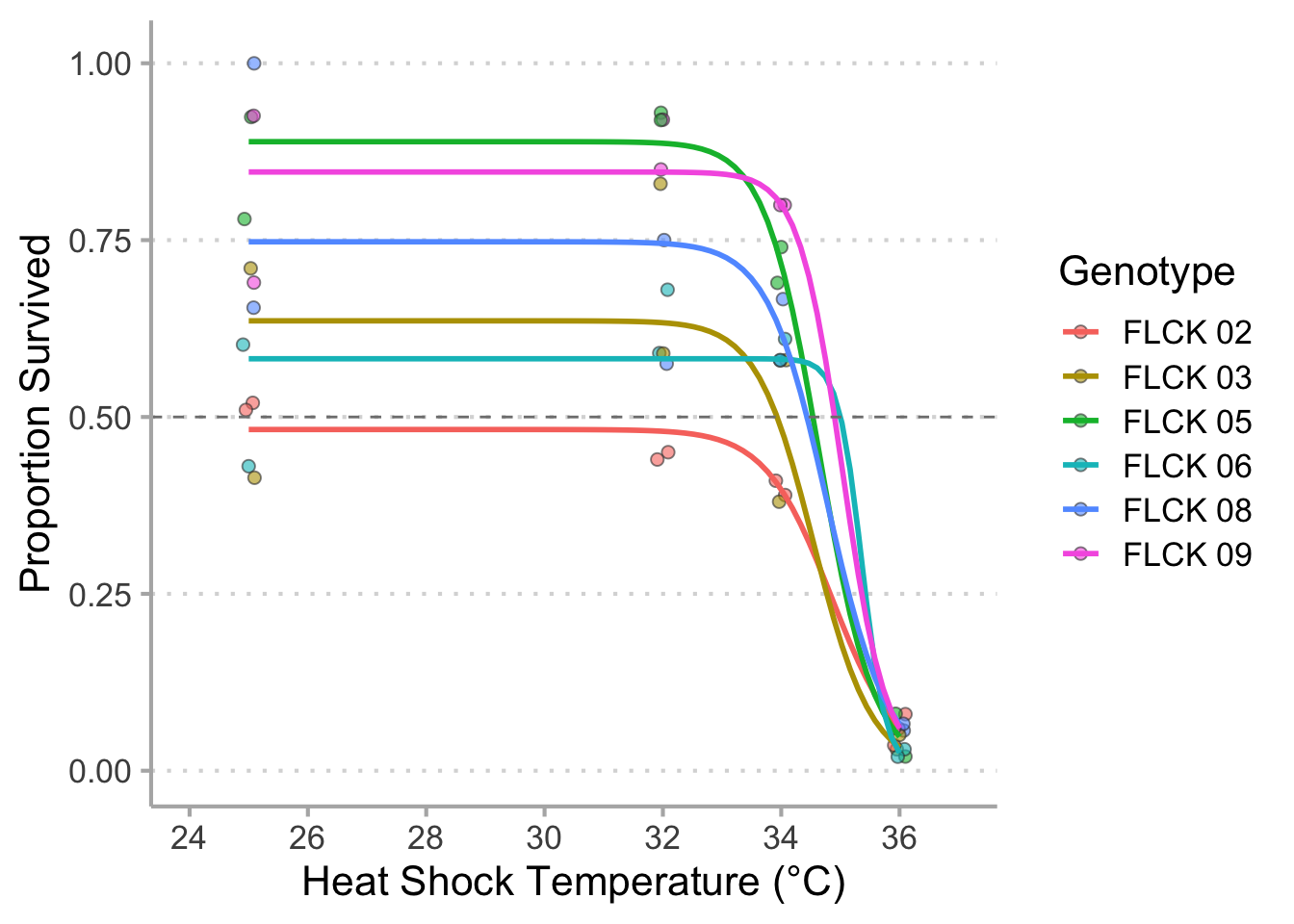
# Plot survival curve for one genotype (FLCK)------------------------------------------
surv %>%
filter(str_detect(Genotype, "FLCK")) %>%
mutate(Prop_Hatched = Hatched_48/Eggs) %>%
ggplot(aes(x = Temperature,
y = Prop_Hatched,
color = Genotype,
fill = Genotype)) +
geom_jitter(width = 0.1,
shape = 21,
alpha = 0.6,
size = 2,
color = "grey23") +
geom_smooth(method = drm,
method.args = list(fct = LL.3()),
se = FALSE) +
geom_hline(yintercept = 0.5,
color = "grey50",
linetype = 2) +
labs(x = "Heat Shock Temperature (°C)",
y = "Proportion Survived") +
scale_y_continuous(limits = c(0, 1.01),
breaks = seq(from = 0, to = 1, by = 0.25)) +
scale_x_continuous(limits = c(24, 37),
breaks = seq(from = 24, to = 38, by = 2)) +
theme_classic(base_size = 16) +
theme(panel.grid.major.y = element_line(color = "grey85",
linetype = 3),
axis.line = element_line(color = "grey70"),
axis.ticks = element_line(color = "grey70"))
# `geom_smooth()` using formula 'y ~ x'
# ggsave("flck_final.png",
# height = 6,
# width = 9)
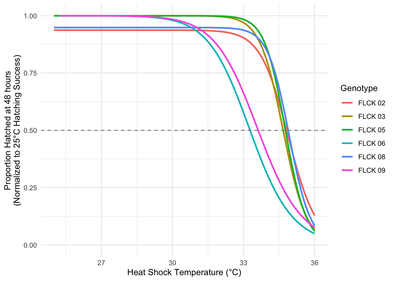
# Renormalize to 25°C hatching success ----------------------------------------
surv %>%
filter(str_detect(Genotype, "FLCK")) %>%
group_by(Genotype, Temperature) %>%
summarise(Prop_Hatched = sum(Hatched_48)/sum(Eggs)) %>%
mutate(Prop_Hatched_norm = Prop_Hatched/Prop_Hatched[Temperature == 25]) %>%
ggplot(aes(x = Temperature,
y = Prop_Hatched_norm,
color = Genotype)) +
geom_smooth(method = drm,
method.args = list(fct = LL.3()),
se = FALSE) +
geom_hline(yintercept = 0.5,
color = "grey50",
linetype = 2) +
labs(x = "Heat Shock Temperature (°C)",
y = "Proportion Hatched at 48 hours\n(Normalized to 25°C Hatching Success)") +
ylim(c(0, 1)) +
theme_minimal()
# `summarise()` has grouped output by 'Genotype'. You can override using the
# `.groups` argument.
# `geom_smooth()` using formula 'y ~ x'
# Warning: Removed 6 rows containing non-finite values (stat_smooth).
# Warning in pt(x, df.residual(object)): NaNs produced
# Warning in pt(x, df.residual(object)): NaNs produced
# Warning in pt(x, df.residual(object)): NaNs produced
# Warning in pt(x, df.residual(object)): NaNs produced
# Warning in sqrt(resVar): NaNs produced
# Warning in sqrt(diag(varMat)): NaNs produced
# Warning in sqrt(resVar): NaNs produced
# Warning in sqrt(diag(varMat)): NaNs produced
# Warning: Removed 4 rows containing missing values (geom_smooth).
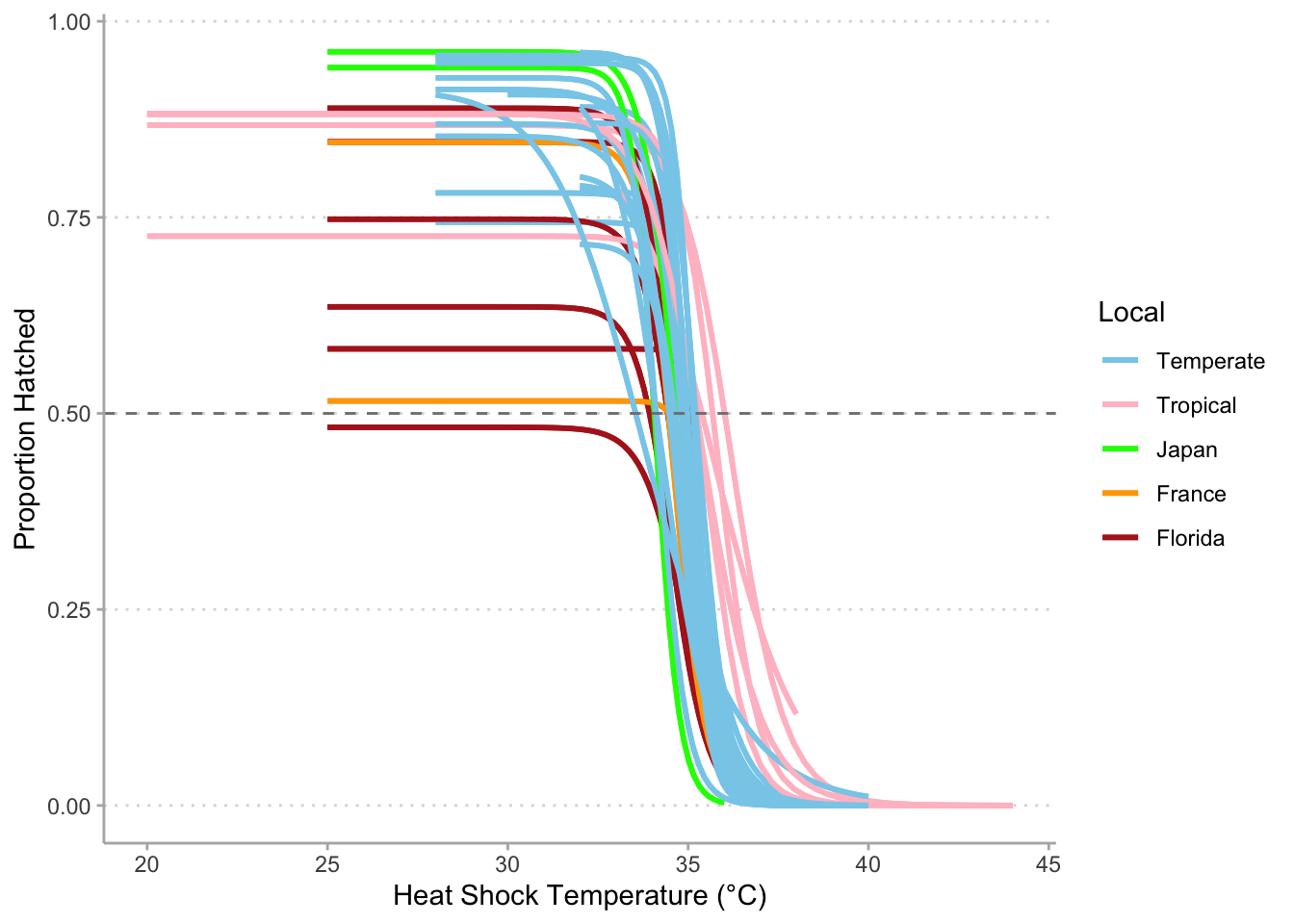
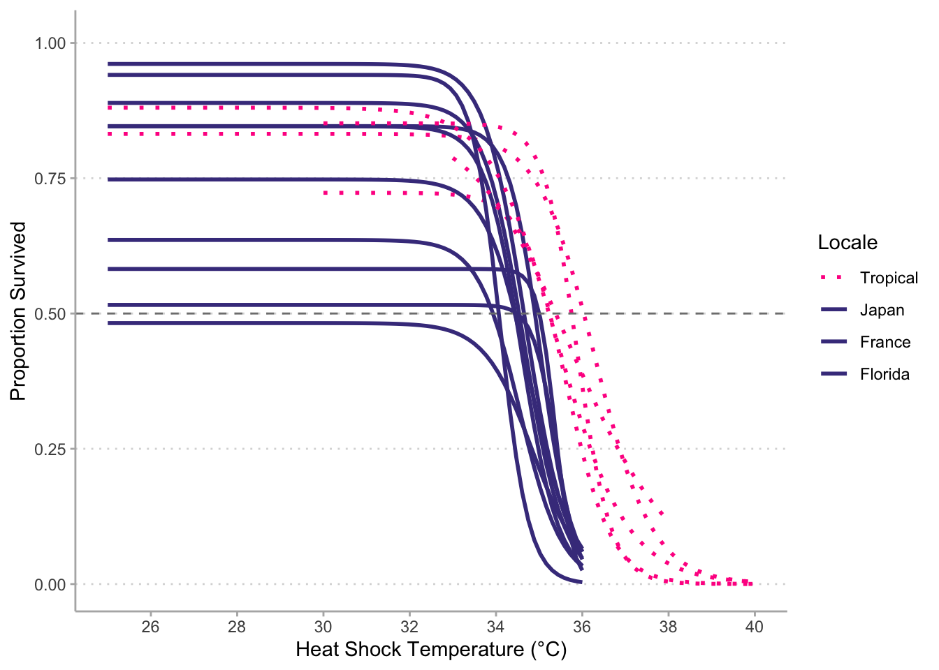
#Combined surv curve-----------------------------------------------------------
surv %>%
  mutate(region = ifelse(is.na (region),
                         case_when(str_detect(Genotype, "FLCK") ~ "Florida",
                                   str_detect(Genotype, "FR") ~ "France",
                                   str_detect(Genotype, "JP") ~ "Japan"),
                         str_to_sentence(region))) %>%
  mutate(region = factor(region, levels = c("Temperate", "Tropical",
                                            "Japan", "France", "Florida"))) %>%
  filter(!str_detect(Genotype, "Canton") &
           !str_detect(Genotype, "X")) %>%
  ggplot(aes(x = Temperature,
             y = Hatched_48/Eggs,
             color = region)) +
  geom_smooth (aes(group = Genotype),
               method = drm,
               method.args = list(fct = LL.3()),
               se = FALSE) +
  geom_smooth (aes(group = Genotype),
               method = drm,
               method.args = list(fct = LL.3()),
               se = FALSE) +
  geom_hline (yintercept = 0.50,
              color = "grey50",
              linetype = 2) +
  scale_color_manual(values = c("skyblue",
                                "pink",
                                "green",
                                "orange",
                                "firebrick"),
                     name = "Local") +
  labs(x = "Heat Shock Temperature (°C)",
       y = "Proportion Hatched") +
  theme_classic() +
  theme(panel.grid.major.y = element_line(color = "grey85",
                                          linetype = 3),
        axis.line = element_line(color = "grey70"),
        axis.ticks = element_line(color = "grey70"))
# `geom_smooth()` using formula 'y ~ x'
# `geom_smooth()` using formula 'y ~ x'
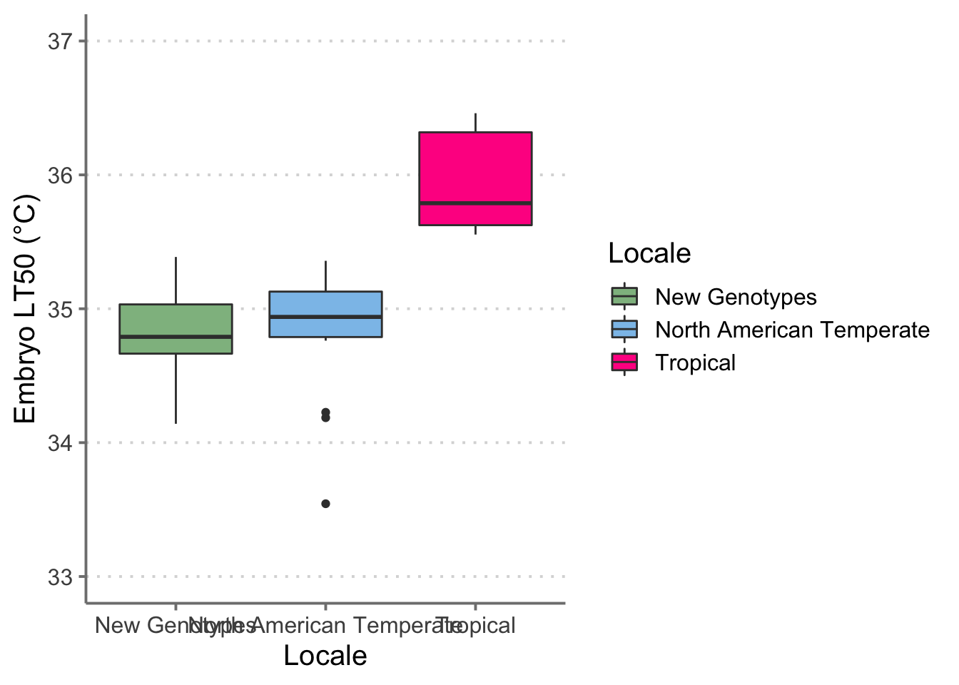
# Box plot of LT50s (Japan together)------------------------------------------------------------
lt_surv_curv %>%
  filter(!str_detect(Genotype, "X")) %>%
  mutate(region = case_when(str_detect(Genotype, "FLCK") ~ "New Genotypes",
                            str_detect(Genotype, "VT") |
                              str_detect(Genotype, "BEA") |
                              str_detect(Genotype, "RFM") ~ "North American Temperate",
                            str_detect(Genotype, "JP") ~ "New Genotypes",
                            str_detect(Genotype, "FR") ~ "New Genotypes",
                            TRUE ~ "Tropical")) %>%
  ggplot() +
  geom_boxplot(aes(x = region,
                   y = lt_50,
                   fill = region,
                   color = region)) +
  scale_fill_manual("Locale", values = c( "New Genotypes" = "darkseagreen",
                               "North American Temperate" = "#8CC2EA",
                               "Tropical" = "#FF2E91")) +
  scale_color_manual("Locale", values = c("New Genotypes" = "grey23",
                                "North American Temperate" = "grey23",
                                "Tropical" = "grey23")) +
  labs(x = "Locale",
       y = "Embryo LT50 (°C)") +
  ylim(c(33, 37)) +
  theme_classic(base_size = 15) +
  theme(panel.grid.major.y = element_line(color = "grey85",
                                          linetype = 3),
        axis.line = element_line(color = "grey50"),
        axis.ticks = element_line(color = "grey50"))
# ggsave("boxplot_final_pres.png",
# height = 6,
# width = 9)
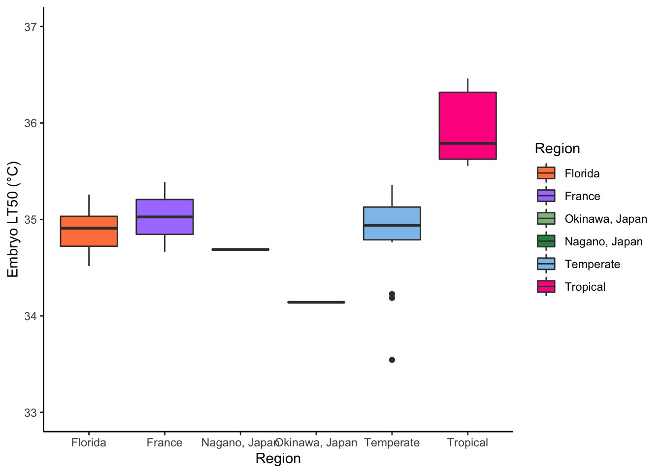
#Box Plot LT50s (Japan Split)--------------------------------------------------
lt_surv_curv %>%
filter(!str_detect(Genotype, "X")) %>%
mutate(region = case_when(str_detect(Genotype, "FLCK") ~ "Florida",
str_detect(Genotype, "VT") |
str_detect(Genotype, "BEA") |
str_detect(Genotype, "RFM") ~ "Temperate",
str_detect(Genotype, "JPOK") ~ "Okinawa, Japan",
str_detect(Genotype, "JPSC") ~ "Nagano, Japan",
str_detect(Genotype, "FR") ~ "France",
TRUE ~ "Tropical")) %>%
ggplot() +
geom_boxplot(aes(x = region,
y = lt_50,
fill = region,
color = region)) +
scale_fill_manual("Region", values = c("Florida" = "sienna1",
"France" = "mediumpurple1",
"Okinawa, Japan" = "darkseagreen",
"Nagano, Japan" = "seagreen",
"Temperate" = "#8CC2EA",
"Tropical" = "#FF2D8F")) +
scale_color_manual("Region", values = c("Florida" = "grey23",
"France" = "grey23",
"Okinawa, Japan" = "grey23",
"Nagano, Japan" = "grey23",
"Temperate" = "grey23",
"Tropical" = "grey23")) +
labs(x = "Region",
y = "Embryo LT50 (°C)") +
ylim(c(33, 37)) +
theme_classic()
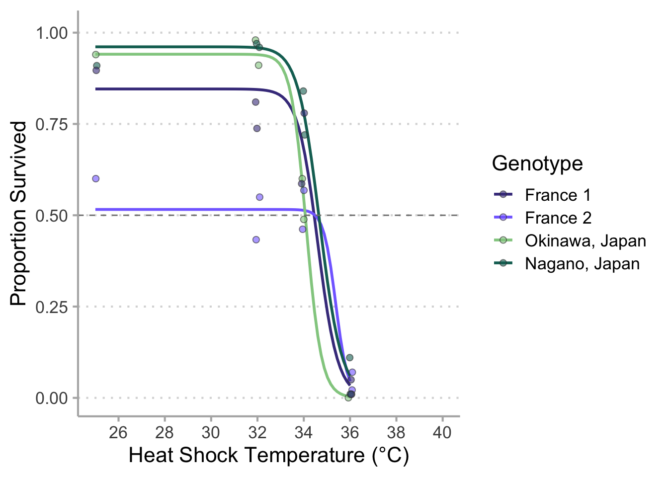
# New data----------------------------------------------------------------------
surv %>%
  filter(Genotype == "FRMO-01" |
           Genotype == "FRMO-02" |
           Genotype == "JPSC" |
           Genotype == "JPOK") %>%
  ggplot(aes(x = Temperature,
             y = Hatched_48/Eggs,
             color = Genotype,
             fill = Genotype)) +
  geom_smooth (method = drm,
               method.args = list(fct = LL.3()),
               se = FALSE) +
  geom_jitter(width = 0.1,
              shape = 21,
              alpha = 0.6,
              size = 2,
              color = "grey23") +
  geom_hline (yintercept = 0.50,
              color = "grey50",
              linetype = 2) +
  scale_color_manual(values = c("slateblue4",
                                "slateblue1",
                                "#92CC8F",
                                "#136F63"),
                     labels = c("France 1",
                                "France 2",
                                "Okinawa, Japan",
                                "Nagano, Japan")) +
  scale_fill_manual(values = c("slateblue4",
                               "slateblue1",
                               "#92CC8F",
                               "#136F63"),
                    labels = c("France 1",
                               "France 2",
                               "Okinawa, Japan",
                               "Nagano, Japan")) +
  scale_x_continuous(limits = c(25, 40),
                     breaks = seq(from = 26, to = 40, by = 2)) +
  scale_y_continuous(limits = c(0, 1.01),
                     breaks = seq(from = 0, to = 1, by = 0.25)) +
  labs(x = "Heat Shock Temperature (°C)",
       y = "Proportion Survived") +
  theme_classic(base_size = 16) +
  theme(panel.grid.major.y = element_line(color = "grey85",
                                          linetype = 3),
        axis.line = element_line(color = "grey70"),
        axis.ticks = element_line(color = "grey70"))
# `geom_smooth()` using formula 'y ~ x'
# Warning: Removed 4 rows containing missing values (geom_point).
# ggsave("fr_jp_final.png",
#        height = 6,
#        width = 9)

# Temperate vs new data---------------------------------------------------------
surv %>%
  mutate(region = ifelse(is.na (region),
                         case_when(str_detect(Genotype, "FLCK") ~ "Florida",
                                   str_detect(Genotype, "FR") ~ "France",
                                   str_detect(Genotype, "JPOK") ~ "Okinawa",
                                   str_detect(Genotype, "JPSC") ~ "Nagano"),
                         str_to_sentence(region))) %>%
  mutate(region = factor(region, levels = c("Temperate", "Tropical",
                                            "Japan", "France", "Florida"))) %>%
  filter(!str_detect(Genotype, "Canton") &
           !str_detect(Genotype, "X") &
           !str_detect(region, "Tropical")) %>%
  ggplot(aes(x = Temperature,
             y = Hatched_48/Eggs,
             color = region,
             linetype = region)) +
  geom_smooth (aes(group = Genotype),
               method = drm,
               method.args = list(fct = LL.3()),
               se = FALSE) +
  geom_hline (yintercept = 0.50,
              color = "grey50",
              linetype = 2) +
  scale_color_manual(values = c("#8CC2EA",
                                "slateblue4",
                                "slateblue4",
                                "slateblue4",
                                "slateblue4"),
                     name = "Local") +
  scale_linetype_manual(values = c(3,
                                   1,
                                   1,
                                   1)) +
  scale_x_continuous(limits = c(25, 40)) +
  labs(x = "Heat Shock Temperature (°C)",
       y = "Proportion Hatched") +
  theme_classic() +
  theme(panel.grid.major.y = element_line(color = "grey85",
                                          linetype = 3),
        axis.line = element_line(color = "grey70"),
        axis.ticks = element_line(color = "grey70")) +
  theme(axis.line.y = element_blank(),
        legend.position = "none")
# `geom_smooth()` using formula 'y ~ x'
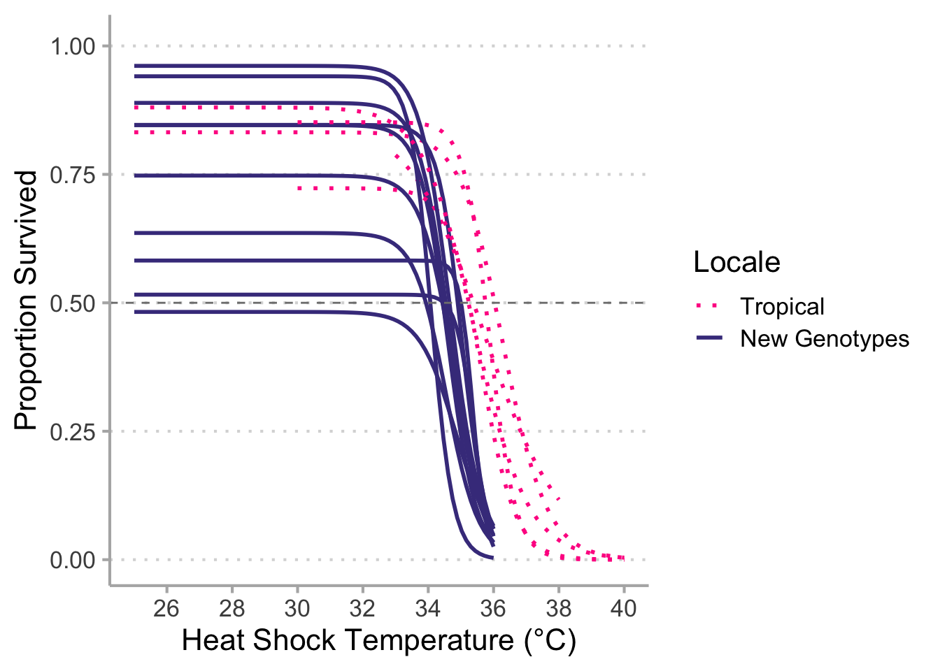
# Tropical vs new data----------------------------------------------------------
surv %>%
  mutate(region = ifelse(is.na (region),
                         case_when(str_detect(Genotype, "FLCK") ~ "Florida",
                                   str_detect(Genotype, "FR") ~ "France",
                                   str_detect(Genotype, "JP") ~ "Japan"),
                         str_to_sentence(region))) %>%
  mutate(region = factor(region, levels = c("Temperate", "Tropical",
                                            "Japan", "France", "Florida"))) %>%
  filter(!str_detect(Genotype, "Canton") &
           !str_detect(Genotype, "X") &
           !str_detect(region, "Temperate")) %>%
  ggplot(aes(x = Temperature,
             y = Hatched_48/Eggs,
             color = region,
             linetype = region)) +
  geom_smooth (aes(group = Genotype),
               method = drm,
               method.args = list(fct = LL.3()),
               se = FALSE) +
  scale_color_manual(values = c("#FF2E91",
                                "slateblue4",
                                "slateblue4",
                                "slateblue4"),
                     name = "Locale") +
  scale_linetype_manual(values = c(3,
                                   1,
                                   1,
                                   1),
                        name = "Locale") +
  geom_hline (yintercept = 0.50,
              color = "grey50",
              linetype = 2) +
  scale_x_continuous(limits = c(25, 40),
                     breaks = seq(from = 26, to = 40, by = 2)) +
  scale_y_continuous(limits = c(0, 1.01),
                     breaks = seq(from = 0, to = 1, by = 0.25)) +
  labs(x = "Heat Shock Temperature (°C)",
       y = "Proportion Survived") +
  theme_classic() +
  theme(panel.grid.major.y = element_line(color = "grey85",
                                          linetype = 3),
        axis.line = element_line(color = "grey70"),
        axis.ticks = element_line(color = "grey70"))
# `geom_smooth()` using formula 'y ~ x'
# Warning: Removed 39 rows containing non-finite values (stat_smooth).
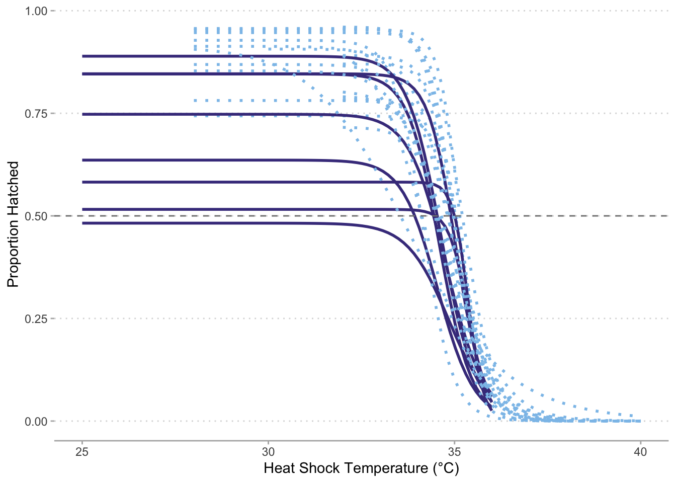
# Correct legends --------------------------------------------------------------
surv %>%
  mutate(region = ifelse(is.na (region),
                         case_when(str_detect(Genotype, "FLCK") |
                                   str_detect(Genotype, "FR") |
                                   str_detect(Genotype, "JP") ~ "New Genotypes"),
                         str_to_sentence(region))) %>%
  mutate(region = factor(region, levels = c("Temperate", "Tropical",
                                            "New Genotypes"))) %>%
  filter(!str_detect(Genotype, "Canton") &
           !str_detect(Genotype, "X") &
           !str_detect(region, "Temperate")) %>%
  ggplot(aes(x = Temperature,
             y = Hatched_48/Eggs,
             color = region,
             linetype = region)) +
  geom_smooth (aes(group = Genotype),
               method = drm,
               method.args = list(fct = LL.3()),
               se = FALSE) +
  scale_color_manual(values = c("#FF2E91", "slateblue4"),
                     name = "Locale") +
  scale_linetype_manual(values = c(3, 1),
                        name = "Locale") +
  geom_hline (yintercept = 0.50,
              color = "grey50",
              linetype = 2) +
  scale_x_continuous(limits = c(25, 40),
                     breaks = seq(from = 26, to = 40, by = 2)) +
  scale_y_continuous(limits = c(0, 1.01),
                     breaks = seq(from = 0, to = 1, by = 0.25)) +
  labs(x = "Heat Shock Temperature (°C)",
       y = "Proportion Survived") +
  theme_classic(base_size = 16) +
  theme(panel.grid.major.y = element_line(color = "grey85",
                                          linetype = 3),
        axis.line = element_line(color = "grey70"),
        axis.ticks = element_line(color = "grey70"))
# `geom_smooth()` using formula 'y ~ x'
# Warning: Removed 39 rows containing non-finite values (stat_smooth).
# ggsave("new_data_vs_tropical_final.png",
# height = 6,
# width = 9)
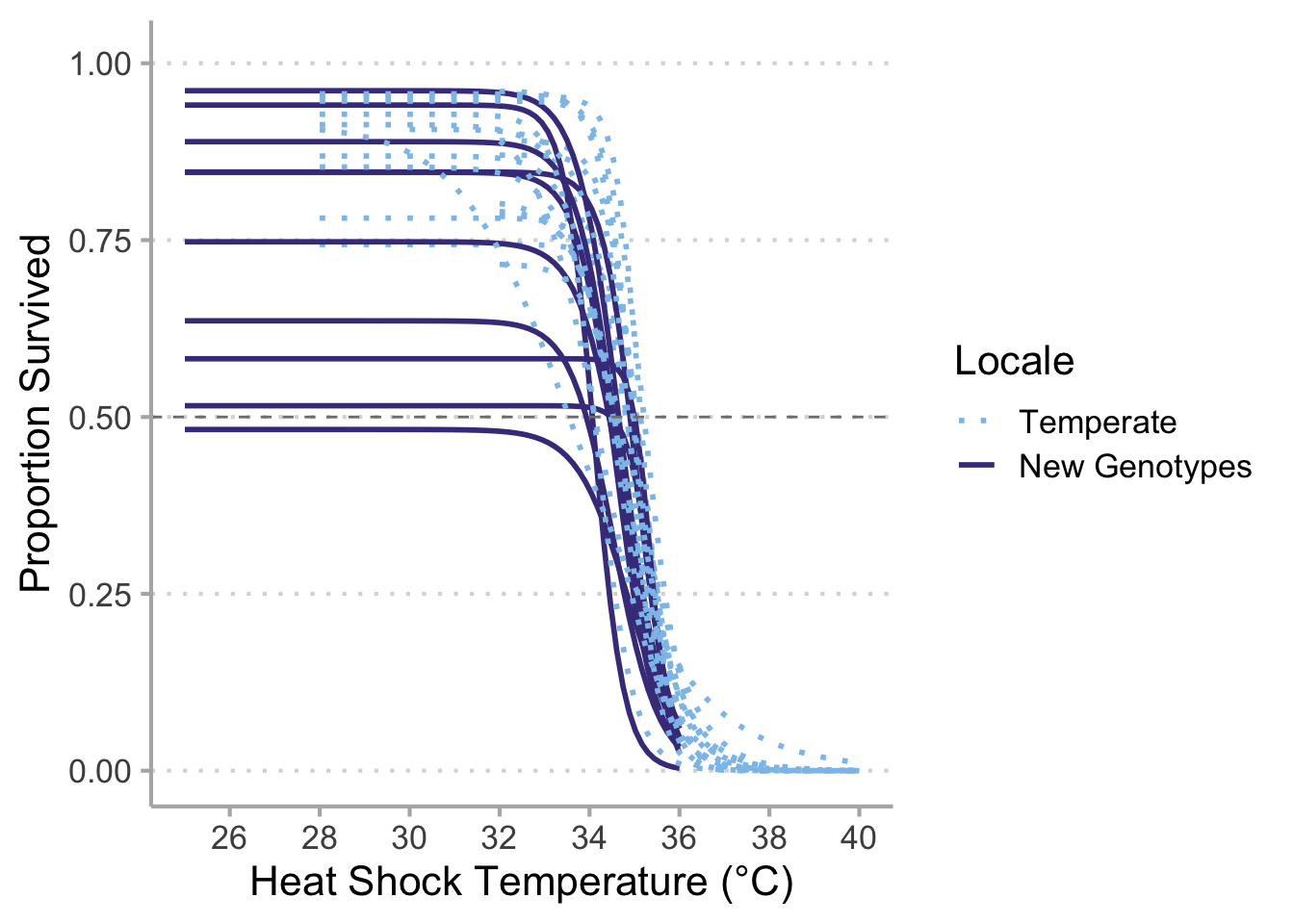
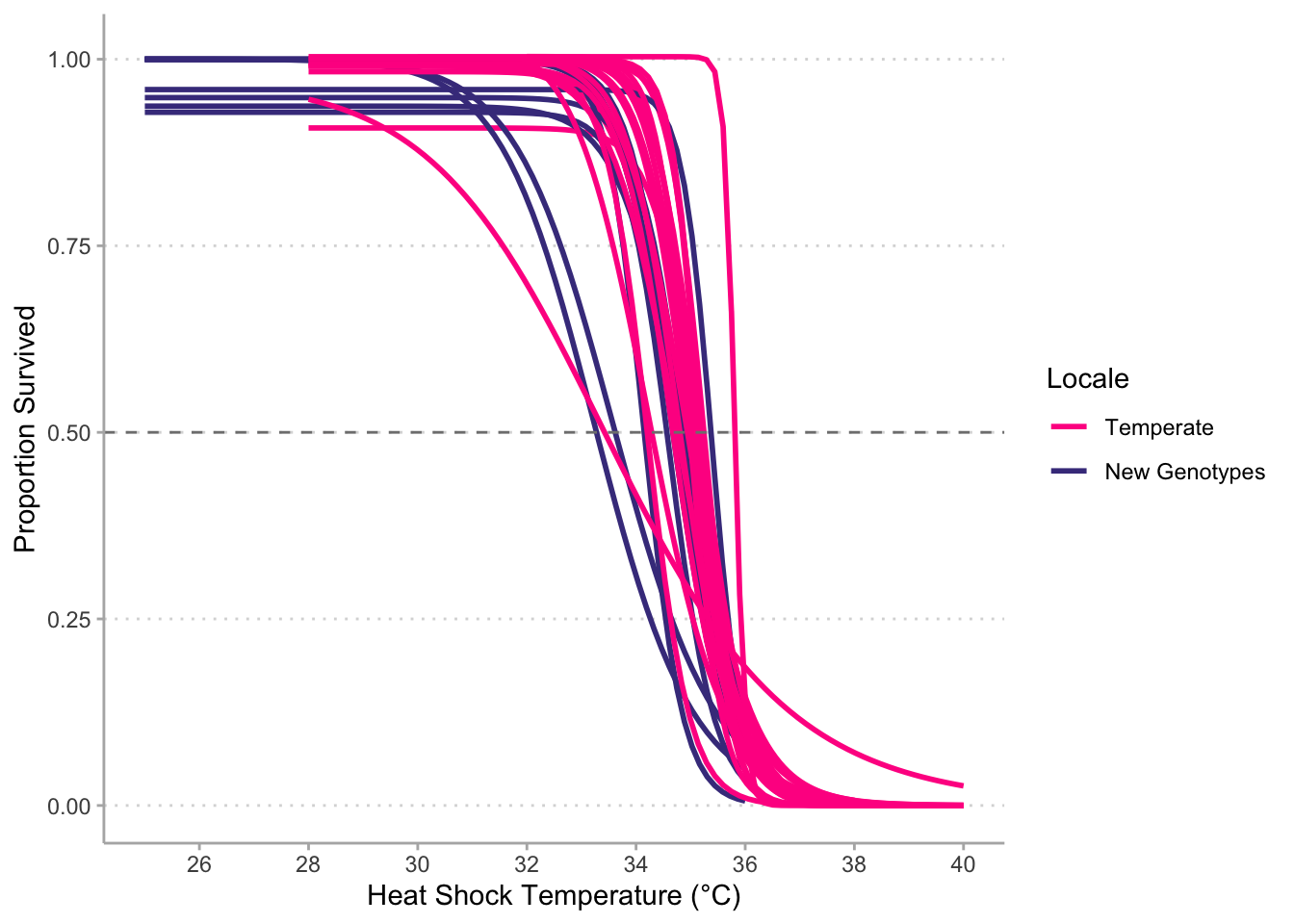
# New and Temperate ------------------------------------------------------------
surv %>%
mutate(region = ifelse(is.na (region),
case_when(str_detect(Genotype, "FLCK") |
str_detect(Genotype, "FR") |
str_detect(Genotype, "JP") ~ "New Genotypes"),
str_to_sentence(region))) %>%
mutate(region = factor(region, levels = c("Temperate", "Tropical",
"New Genotypes"))) %>%
filter(!str_detect(Genotype, "Canton") &
!str_detect(Genotype, "X") &
!str_detect(region, "Tropical")) %>%
ggplot(aes(x = Temperature,
y = Hatched_48/Eggs,
color = region,
linetype = region)) +
geom_smooth (aes(group = Genotype),
method = drm,
method.args = list(fct = LL.3()),
se = FALSE) +
scale_color_manual(values = c("#8CC2EA", "slateblue4"),
name = "Locale") +
scale_linetype_manual(values = c(3, 1),
name = "Locale") +
geom_hline (yintercept = 0.50,
color = "grey50",
linetype = 2) +
scale_x_continuous(limits = c(25, 40),
breaks = seq(from = 26, to = 40, by = 2)) +
scale_y_continuous(limits = c(0, 1.01),
breaks = seq(from = 0, to = 1, by = 0.25)) +
labs(x = "Heat Shock Temperature (°C)",
y = "Proportion Survived") +
theme_classic(base_size = 16) +
theme(panel.grid.major.y = element_line(color = "grey85",
linetype = 3),
axis.line = element_line(color = "grey70"),
axis.ticks = element_line(color = "grey70"))
# `geom_smooth()` using formula 'y ~ x'
# ggsave("new_data_vs_temperate_final.png",
# height = 6,
# width = 9)
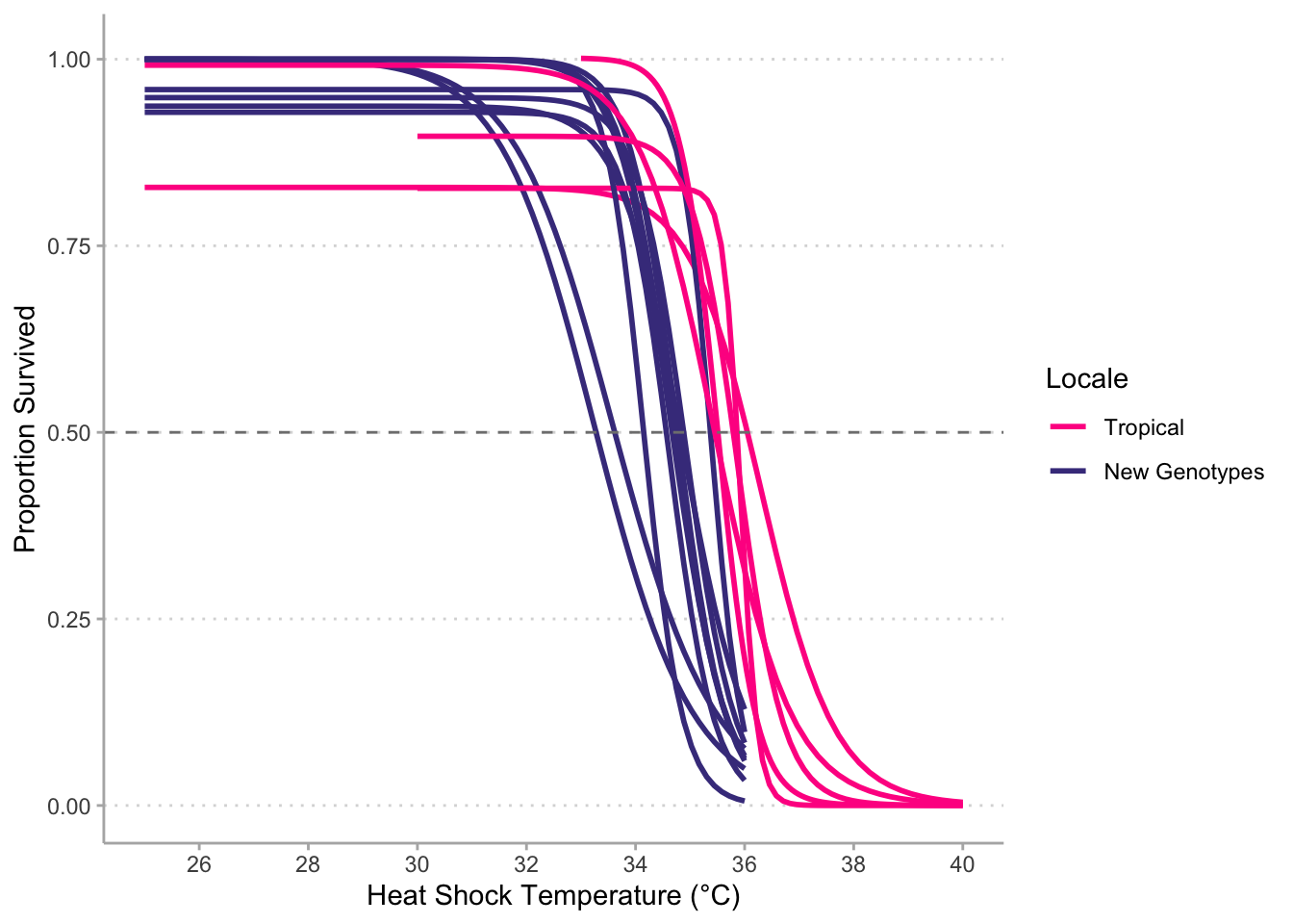
# Normalized to 25°C survival (tropical) --------------------------------------
surv %>%
filter(!str_detect(Genotype, "Canton") &
!str_detect(Genotype, "X")) %>%
group_by(Genotype, Temperature) %>%
summarise(Prop_Hatched = sum(Hatched_48)/sum(Eggs)) %>%
mutate(Prop_Hatched_norm = Prop_Hatched/Prop_Hatched[Temperature == min(Temperature)]) %>%
mutate(region = case_when(str_detect(Genotype, "FLCK") |
str_detect(Genotype, "FR") |
str_detect(Genotype, "JP") ~ "New Genotypes",
str_detect(Genotype, "FLCK") |
str_detect(Genotype, "MU") |
str_detect(Genotype, "CH") |
str_detect(Genotype, "GH") |
str_detect(Genotype, "SK") |
str_detect(Genotype, "GU") ~ "Tropical",
str_detect(Genotype, "VTECK_") |
str_detect(Genotype, "BEA") |
str_detect(Genotype, "RFM") ~ "Temperate")) %>%
mutate(region = factor(region, levels = c("Temperate", "Tropical",
"New Genotypes"))) %>%
filter(region != "Temperate") %>%
ggplot(aes(x = Temperature,
y = Prop_Hatched_norm,
color = region)) +
geom_smooth(aes(group = Genotype),
method = drm,
method.args = list(fct = LL.3()),
se = FALSE) +
scale_color_manual(values = c("#FF2E91", "slateblue4"),
name = "Locale") +
scale_linetype_manual(values = c(3, 1),
name = "Locale") +
geom_hline (yintercept = 0.50,
color = "grey50",
linetype = 2) +
scale_x_continuous(limits = c(25, 40),
breaks = seq(from = 26, to = 40, by = 2)) +
scale_y_continuous(limits = c(0, 1.01),
breaks = seq(from = 0, to = 1, by = 0.25)) +
labs(x = "Heat Shock Temperature (°C)",
y = "Proportion Survived") +
theme_classic() +
theme(panel.grid.major.y = element_line(color = "grey85",
linetype = 3),
axis.line = element_line(color = "grey70"),
axis.ticks = element_line(color = "grey70"))
# `summarise()` has grouped output by 'Genotype'. You can override using the
# `.groups` argument.
# `geom_smooth()` using formula 'y ~ x'
# Warning: Removed 18 rows containing non-finite values (stat_smooth).
# Warning in pt(x, df.residual(object)): NaNs produced
# Warning in pt(x, df.residual(object)): NaNs produced
# Warning in pt(x, df.residual(object)): NaNs produced
# Warning in pt(x, df.residual(object)): NaNs produced
# Warning in sqrt(resVar): NaNs produced
# Warning in sqrt(diag(varMat)): NaNs produced
# Warning in sqrt(resVar): NaNs produced
# Warning in sqrt(diag(varMat)): NaNs produced
# Warning in pt(x, df.residual(object)): NaNs produced
# Warning in pt(x, df.residual(object)): NaNs produced
# Warning in pt(x, df.residual(object)): NaNs produced
# Warning in pt(x, df.residual(object)): NaNs produced
# Normalized to 25°C survival (temperate) --------------------------------------
surv %>%
  filter(!str_detect(Genotype, "Canton") &
           !str_detect(Genotype, "X")) %>%
  group_by(Genotype, Temperature) %>%
  summarise(Prop_Hatched = sum(Hatched_48)/sum(Eggs)) %>%
  mutate(Prop_Hatched_norm = Prop_Hatched/Prop_Hatched[Temperature == min(Temperature)]) %>%
  mutate(region = case_when(str_detect(Genotype, "VTECK_") |
                              str_detect(Genotype, "BEA") |
                              str_detect(Genotype, "RFM") ~ "Temperate",
                            str_detect(Genotype, "FLCK") |
                              str_detect(Genotype, "FR") |
                              str_detect(Genotype, "JP") ~ "New Genotypes",
                            str_detect(Genotype, "FLCK") |
                              str_detect(Genotype, "MU") |
                              str_detect(Genotype, "CH") |
                              str_detect(Genotype, "GH") |
                              str_detect(Genotype, "SK") |
                              str_detect(Genotype, "GU") ~ "Tropical")) %>%
  mutate(region = factor(region, levels = c("Temperate", "Tropical",
                                            "New Genotypes"))) %>%
  filter(region != "Tropical") %>%
  ggplot(aes(x = Temperature,
             y = Prop_Hatched_norm,
             color = region)) +
  geom_smooth(aes(group = Genotype),
              method = drm,
              method.args = list(fct = LL.3()),
              se = FALSE) +
  scale_color_manual(values = c("#FF2E91", "slateblue4"),
                     name = "Locale") +
  scale_linetype_manual(values = c(3, 1),
                        name = "Locale") +
  geom_hline (yintercept = 0.50,
              color = "grey50",
              linetype = 2) +
  scale_x_continuous(limits = c(25, 40),
                     breaks = seq(from = 26, to = 40, by = 2)) +
  scale_y_continuous(limits = c(0, 1.01),
                     breaks = seq(from = 0, to = 1, by = 0.25)) +
  labs(x = "Heat Shock Temperature (°C)",
       y = "Proportion Survived") +
  theme_classic() +
  theme(panel.grid.major.y = element_line(color = "grey85",
                                          linetype = 3),
        axis.line = element_line(color = "grey70"),
        axis.ticks = element_line(color = "grey70"))
# `summarise()` has grouped output by 'Genotype'. You can override using the
# `.groups` argument.
# `geom_smooth()` using formula 'y ~ x'
# Warning: Removed 15 rows containing non-finite values (stat_smooth).
# NaNs produced
# NaNs produced
# NaNs produced
# NaNs produced
# Warning in sqrt(resVar): NaNs produced
# Warning in sqrt(diag(varMat)): NaNs produced
# Warning in sqrt(resVar): NaNs produced
# Warning in sqrt(diag(varMat)): NaNs produced
# Warning in pt(x, df.residual(object)): NaNs produced

# Warning in pt(x, df.residual(object)): NaNs produced

# Warning in pt(x, df.residual(object)): NaNs produced

# Warning in pt(x, df.residual(object)): NaNs produced
# ------------------------------------------------------------------------------
# Stat time
lts_df <- lt_surv_curv  %>%
  filter(!str_detect(Genotype, "X")) %>%
  mutate(locale = case_when(str_detect(Genotype, "FLCK") ~ "Florida",
                            str_detect(Genotype, "VT") |
                              str_detect(Genotype, "BEA") |
                              str_detect(Genotype, "RFM") ~ "Temperate",
                            str_detect(Genotype, "JP") ~ "Japan",
                            str_detect(Genotype, "FR") ~ "France",
                            TRUE ~ "Tropical"))

# ANOVA regular style
mod_aov <- aov(lt_50 ~ locale, data = lts_df)
summary(mod_aov)
#             Df Sum Sq Mean Sq F value   Pr(>F)
# locale       4  5.633  1.4083   8.044 0.000172 ***
# Residuals   29  5.077  0.1751
# ---
# Signif. codes:  0 '***' 0.001 '**' 0.01 '*' 0.05 '.' 0.1 ' ' 1

TukeyHSD(mod_aov)
#   Tukey multiple comparisons of means
#     95% family-wise confidence level
#
# Fit: aov(formula = lt_50 ~ locale, data = lts_df)
#
# $locale
#                           diff         lwr       upr     p adj
# France-Florida      0.13823093 -0.85483551 1.1312974 0.9940442
# Japan-Florida      -0.47281643 -1.46588288 0.5202500 0.6423868
# Temperate-Florida  -0.02686905 -0.59643172 0.5426936 0.9999152
# Tropical-Florida    1.06164915  0.32517136 1.7981269 0.0020592
# Japan-France       -0.61104736 -1.82730040 0.6052057 0.5952278
# Temperate-France   -0.16509998 -1.06925269 0.7390527 0.9834059
# Tropical-France     0.92341822 -0.09417207 1.9410085 0.0894335
# Temperate-Japan     0.44594738 -0.45820532 1.3501001 0.6117448
# Tropical-Japan      1.53446558  0.51687529 2.5520559 0.0012293
# Tropical-Temperate  1.08851820  0.47719940 1.6998370 0.0001424

# Combining all new stuff to the same locale
lts_df_new <- lt_surv_curv  %>%
  filter(!str_detect(Genotype, "X")) %>%
  mutate(locale = case_when(str_detect(Genotype, "FLCK") ~ "New Genotype",
                            str_detect(Genotype, "VT") |
                              str_detect(Genotype, "BEA") |
                              str_detect(Genotype, "RFM") ~ "Temperate",
                            str_detect(Genotype, "JP") ~ "New Genotype",
                            str_detect(Genotype, "FR") ~ "New Genotype",
                            TRUE ~ "Tropical"))

# ANOVA regular style
mod_aov_new <- aov(lt_50 ~ locale, data = lts_df_new)
summary(mod_aov_new)
#             Df Sum Sq Mean Sq F value   Pr(>F)
# locale       2  5.193   2.596   14.59 3.43e-05 ***
# Residuals   31  5.518   0.178
# ---
# Signif. codes:  0 '***' 0.001 '**' 0.01 '*' 0.05 '.' 0.1 ' ' 1

TukeyHSD(mod_aov_new)
#   Tukey multiple comparisons of means
#     95% family-wise confidence level
#
# Fit: aov(formula = lt_50 ~ locale, data = lts_df_new)
#
# $locale
#                              diff        lwr       upr     p adj
# Temperate-New Genotype 0.04004805 -0.3656105 0.4457066 0.9680119
# Tropical-New Genotype  1.12856625  0.5598455 1.6972870 0.0000869
# Tropical-Temperate     1.08851820  0.5666243 1.6104121 0.0000427

# Kruskal-Wallis --
mod_aov_ks <- kruskal.test(lt_50 ~ locale, data = lts_df)
mod_aov_ks
#
#   Kruskal-Wallis rank sum test
#
# data:  lt_50 by locale
# Kruskal-Wallis chi-squared = 14.732, df = 4, p-value = 0.005292

pairwise.wilcox.test(x = lts_df$lt_50, g = lts_df$locale)
#
#   Pairwise comparisons using Wilcoxon rank sum exact test
#
# data:  lts_df$lt_50 and lts_df$locale
#
#           Florida France  Japan   Temperate
# France    1.00000 -       -       -
# Japan     1.00000 1.00000 -       -
# Temperate 1.00000 1.00000 0.68571 -
# Tropical  0.03896 0.68571 0.68571 0.00047
#
# P value adjustment method: holm
Catherine & Caleb
# ------------------------------------------------------------------------------
# Catherine & Caleb data
# July 19, 2022
# TS O'Leary
# ------------------------------------------------------------------------------
# Load libraries
require(tidyverse)
# Load data
df <- read_csv("student_data/changes_in_AA.csv")
# Rows: 4 Columns: 3
# ── Column specification ────────────────────────────────────────────────────────
# Delimiter: ","
# chr (2): Adult_Acclimation_State, Direction
# dbl (1): value
#
# ℹ Use `spec()` to retrieve the full column specification for this data.
# ℹ Specify the column types or set `show_col_types = FALSE` to quiet this message.
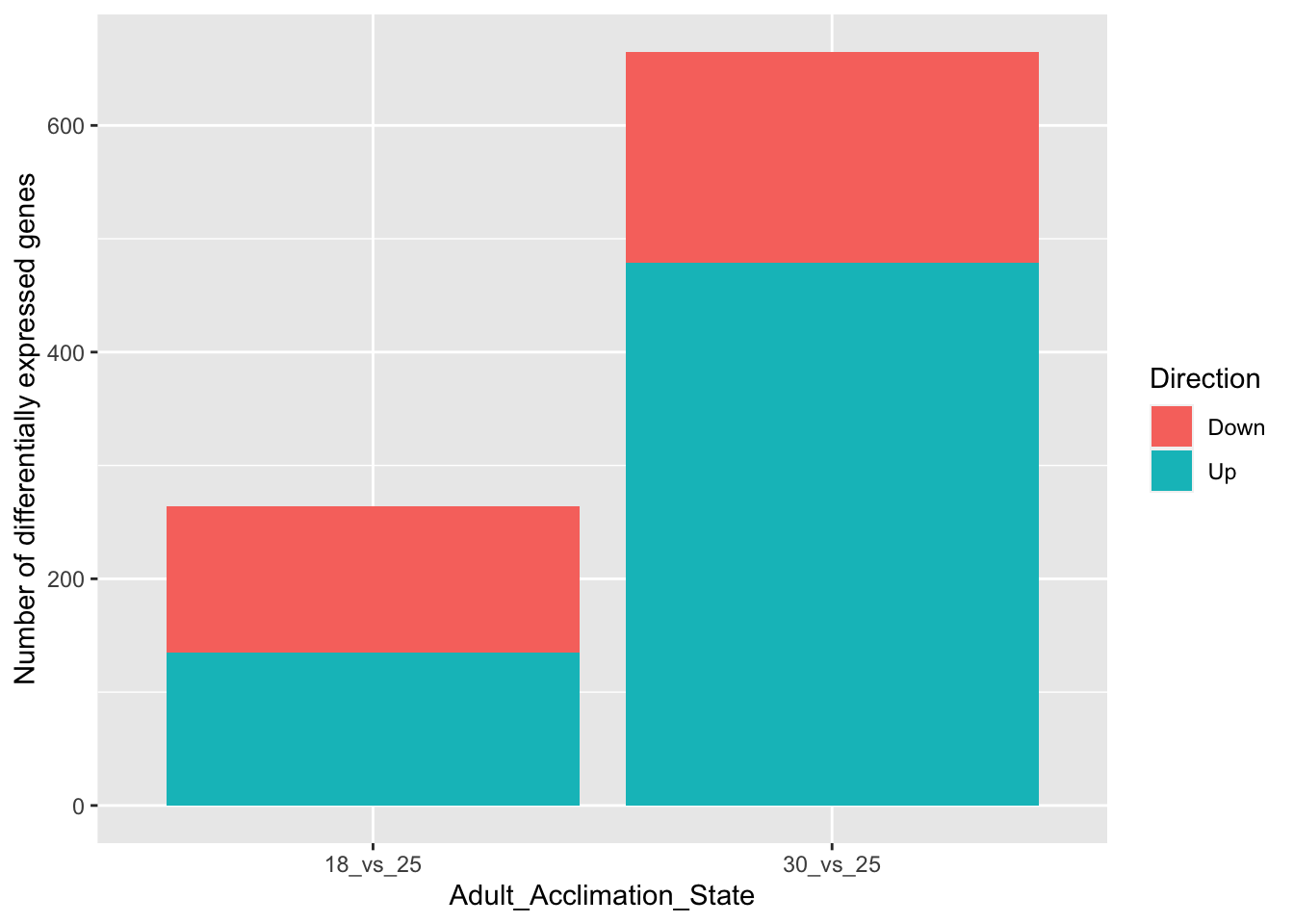
# Plot data
# Minimal plot
ggplot(data = df,
aes(y = value,
x = Adult_Acclimation_State,
fill = Direction)) +
ylab("Number of differentially expressed genes") +
geom_bar(stat = "identity")
# With the position dodge
ggplot(data = df,
       aes(y = value,
           x = Adult_Acclimation_State,
           fill = Direction)) +
  ylab("Number of differentially\nexpressed genes") +
  geom_bar(stat = "identity",
           position = "dodge") +
  theme_classic(base_size = 16)

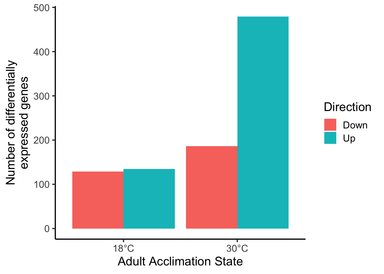
# Those underscores kinda stink
ggplot(data = df,
       aes(y = value,
           x = Adult_Acclimation_State,
           fill = Direction)) +
  geom_bar(stat = "identity",
           position = "dodge") +
  scale_x_discrete(labels = c("18°C", "30°C")) +
  ylab("Number of differentially\nexpressed genes") +
  xlab("Adult Acclimation State") +
  theme_classic(base_size = 16)
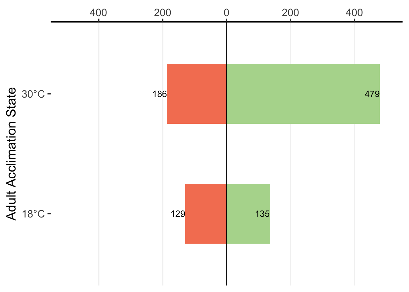
# Okay lets try the thing where the directions depend on the directions
df %>%
  mutate(value = ifelse(Direction == "Down", -value, value)) %>%
  ggplot(aes(x = value,
             y = Adult_Acclimation_State,
             fill = Direction)) +
  geom_bar(stat = "identity",
           position = "identity",
           width = 0.5) +
  geom_vline(xintercept = 0) +
  geom_text(aes(label = abs(value),
                hjust = 1)) +
  scale_y_discrete(labels = c("18°C", "30°C"),
                   name = "Adult Acclimation State") +
  scale_x_continuous(position = "top",
                     name = "Number of differentially expressed genes",
                     limits = c(-500, 500),
                     breaks = seq(from = -400, to = 400, by = 200),
                     labels = abs(seq(from = -400, to = 400, by = 200))) +
  scale_fill_manual(values = c("#F58161", "#B3D89C")) +
  theme_classic(base_size = 16) +
  theme(axis.line.y = element_blank(),
        legend.position = "none",
        panel.grid.major.x = element_line(color = "grey95"),
        axis.title.x = element_blank())
# ggsave("cath_cal_fig.pdf", height = 4, width = 7)
# ------------------------------------------------------------------------------
# Catherine & Caleb data
# July 19, 2022
# TS O'Leary
# ------------------------------------------------------------------------------
# Load data
df <- read_csv("student_data/changes_in_HS_CS_at_AA.csv")
# Rows: 12 Columns: 4
# ── Column specification ────────────────────────────────────────────────────────
# Delimiter: ","
# chr (2): Shock, Direction
# dbl (2): Acclimation_Temp, value
#
# ℹ Use `spec()` to retrieve the full column specification for this data.
# ℹ Specify the column types or set `show_col_types = FALSE` to quiet this message.
# Make plot
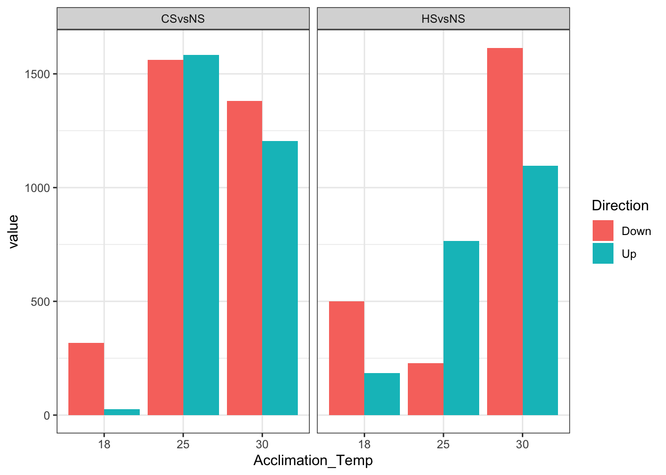
df %>%
mutate(Acclimation_Temp = factor(Acclimation_Temp)) %>%
ggplot(aes(x = Acclimation_Temp,
y = value,
fill = Direction)) +
geom_bar(stat = "identity",
position = "dodge") +
theme_bw() +
facet_wrap(~ Shock)
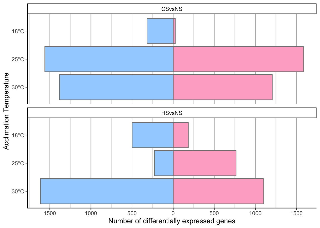
# Make plot
df %>%
  mutate(Acclimation_Temp = factor(paste0(Acclimation_Temp, "°C"),
                                   levels = c("30°C", "25°C", "18°C"))) %>%
  mutate(DEGs = ifelse(Direction == "Up", value, -value)) %>%
  ggplot(aes(y = Acclimation_Temp,
             x = DEGs,
             fill = Direction)) +
  geom_bar(stat = "identity",
           position = "identity",
           color = "grey50") +
  scale_fill_manual(values = c("#a2d2ff", "#ffafcc")) +
  theme_classic() +
  scale_x_continuous(breaks = seq(from = -1500, to = 1500, by = 500),
                     label = abs(seq(from = -1500, to = 1500, by = 500)),
                     name = "Number of differentially expressed genes") +
  ylab("Acclimation Temperature") +
  theme(legend.position = "none",
        panel.grid.major.x = element_line(color = "grey70",
                                        size = 0.5),
        panel.grid.minor.x = element_line(color = "grey90",
                                        size = 0.5)) +
  facet_wrap(~ Shock,
             nrow = 2)
# Change shock name
df %>%
  mutate(Shock = ifelse(Shock == "CSvsNS",
                        "Acute Cold Shock",
                        "Acute Heat Shock")) %>%
  mutate(Acclimation_Temp = factor(paste0(Acclimation_Temp, "°C"),
                                   levels = c("30°C", "25°C", "18°C"))) %>%
  mutate(DEGs = ifelse(Direction == "Up", value, -value)) %>%
  ggplot(aes(y = Acclimation_Temp,
             x = DEGs,
             fill = Direction)) +
  geom_bar(stat = "identity",
           position = "identity",
           color = "grey50") +
  scale_fill_manual(values = c("#a2d2ff", "#ffafcc")) +
  theme_classic() +
  scale_x_continuous(breaks = seq(from = -1500, to = 1500, by = 500),
                     label = abs(seq(from = -1500, to = 1500, by = 500)),
                     name = "Number of differentially expressed genes") +
  ylab("Acclimation Temperature") +
  theme(legend.position = "none",
        panel.grid.major.x = element_line(color = "grey70",
                                        size = 0.5),
        panel.grid.minor.x = element_line(color = "grey90",
                                        size = 0.5)) +
  facet_wrap(~ Shock,
             nrow = 2)

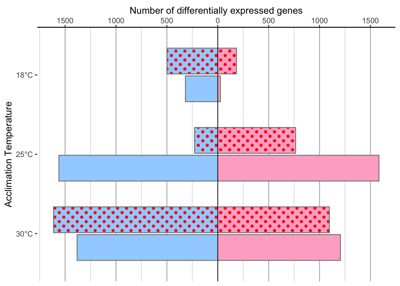
# Dodge by shock
df %>%
  mutate(Shock = ifelse(Shock == "CSvsNS",
                        "Acute Cold Shock",
                        "Acute Heat Shock")) %>%
  mutate(Acclimation_Temp = factor(paste0(Acclimation_Temp, "°C"),
                                   levels = c("30°C", "25°C", "18°C"))) %>%
  mutate(DEGs = ifelse(Direction == "Up", value, -value)) %>%
  ggplot(aes(y = Acclimation_Temp,
             x = DEGs,
             fill = Direction,
             pattern = Shock)) +
  ggpattern::geom_bar_pattern(aes(group = Shock), pattern_color = NA,
                              color = "grey50",
                              width = 0.65,
                              stat = "identity",
                              position = position_dodge(width = 0.7),
                    pattern_fill = "red",
                    pattern_angle = 45,
                    pattern_density = 0.5,
                    pattern_spacing = 0.025,
                    pattern_key_scale_factor = 1) +
  geom_vline(xintercept = 0, color = "grey20") +
  scale_fill_manual(values = c("#a2d2ff", "#ffafcc")) +
  theme_classic(base_size = 12) +
  scale_x_continuous(breaks = seq(from = -1500, to = 1500, by = 500),
                     label = abs(seq(from = -1500, to = 1500, by = 500)),
                     name = "Number of differentially expressed genes",
                     position = "top") +
  ggpattern::scale_pattern_manual(values = c(`Acute Cold Shock` = "none",
                                             `Acute Heat Shock` = "circle")) +
  ylab("Acclimation Temperature") +
  theme(legend.position = "none",
        axis.line.y = element_blank(),
        panel.grid.major.x = element_line(color = "grey70",
                                        size = 0.5),
        panel.grid.minor.x = element_line(color = "grey90",
                                        size = 0.5))
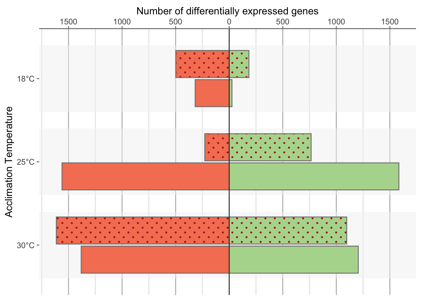
df %>%
  mutate(Shock = ifelse(Shock == "CSvsNS",
                        "Acute Cold Shock",
                        "Acute Heat Shock")) %>%
  mutate(Acclimation_Temp = factor(paste0(Acclimation_Temp, "°C"),
                                   levels = c("30°C", "25°C", "18°C"))) %>%
  mutate(DEGs = ifelse(Direction == "Up", value, -value)) %>%
  ggplot(aes(y = Acclimation_Temp,
             x = DEGs,
             fill = Direction,
             pattern = Shock)) +
  annotate("rect",
           fill = "grey95",
           xmin = -Inf, xmax = Inf,
           ymin = 0.6,
           ymax = 1.4,
           alpha = 0.5) +
  annotate("rect",
           fill = "grey95",
           xmin = -Inf, xmax = Inf,
           ymin = 1.6,
           ymax = 2.4,
           alpha = 0.5) +
    annotate("rect",
           fill = "grey95",
           xmin = -Inf, xmax = Inf,
           ymin = 2.6,
           ymax = 3.4,
           alpha = 0.5) +
  ggpattern::geom_bar_pattern(aes(group = Shock), pattern_color = NA,
                              color = "grey50",
                              width = 0.65,
                              stat = "identity",
                              position = position_dodge(width = 0.7),
                    pattern_fill = "firebrick",
                    pattern_angle = 45,
                    pattern_density = 0.3,
                    pattern_spacing = 0.025,
                    pattern_key_scale_factor = 1) +
  geom_vline(xintercept = 0, color = "grey20") +
  scale_fill_manual(values = c("#F58161", "#B3D89C")) +
  theme_classic(base_size = 12) +
  scale_x_continuous(breaks = seq(from = -1500, to = 1500, by = 500),
                     label = abs(seq(from = -1500, to = 1500, by = 500)),
                     name = "Number of differentially expressed genes",
                     position = "top") +
  ggpattern::scale_pattern_manual(values = c(`Acute Cold Shock` = "none",
                                             `Acute Heat Shock` = "circle")) +
  ylab("Acclimation Temperature") +
  scale_y_discrete(drop = FALSE) +
  theme(legend.position = "none",
        axis.line.y = element_blank(),
        axis.line.x = element_line(color = "grey50"),
        axis.ticks = element_line(color = "grey50"),
        panel.grid.major.x = element_line(color = "grey70",
                                        size = 0.5),
        panel.grid.minor.x = element_line(color = "grey90",
                                        size = 0.5))
Nivea & Sara
# Load packages
require(tidyverse)
require(ggrepel)
# Loading required package: ggrepel
# Load data
df <- read_csv("student_data/send_to_thomas_rRNA.csv")
# Rows: 12545 Columns: 6
# ── Column specification ────────────────────────────────────────────────────────
# Delimiter: ","
# dbl (6): baseMean, log2FoldChange, lfcSE, stat, pvalue, padj
#
# ℹ Use `spec()` to retrieve the full column specification for this data.
# ℹ Specify the column types or set `show_col_types = FALSE` to quiet this message.
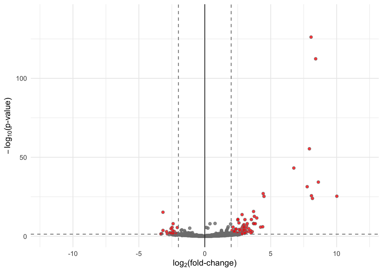
# Make plot
df %>%
filter(!is.na(padj)) %>%
ggplot(mapping = aes(x = log2FoldChange,
y = -log10(padj))) +
geom_point(mapping = aes(fill = padj < 0.05 & abs(log2FoldChange) > 2),
color = "grey50",
shape = 21,
alpha = 0.8) +
geom_hline(yintercept = -log10(0.05),
linetype = "dashed",
color = "grey50") +
geom_vline(xintercept = 0,
color = "grey20") +
geom_vline(xintercept = -2,
linetype = "dashed",
color = "grey50") +
geom_vline(xintercept = 2,
linetype = "dashed",
color = "grey50") +
scale_fill_manual(values = c("grey50", "red")) +
scale_size_manual(values = c(1, 2)) +
xlab(expression(paste(log[2], "(fold-change)"))) +
ylab(expression(paste(-log[10], "(p-value)"))) +
scale_x_continuous(limits = c(-12, 12)) +
ylim(c(0, 140)) +
theme_minimal() +
theme(legend.position = "none")
# ------------------------------------------------------------------------------
# Nivea & Sara -- rRNA depl data -- figs and stuff
# July 21, 2022
# TS O'Leary
# ------------------------------------------------------------------------------
# Load libraries
require(tidyverse)
require(DESeq2)
# Loading required package: DESeq2
# Loading required package: S4Vectors
# Loading required package: stats4
# Loading required package: BiocGenerics
#
# Attaching package: 'BiocGenerics'
# The following objects are masked from 'package:dplyr':
#
# combine, intersect, setdiff, union
# The following objects are masked from 'package:stats':
#
# IQR, mad, sd, var, xtabs
# The following objects are masked from 'package:base':
#
# anyDuplicated, append, as.data.frame, basename, cbind, colnames,
# dirname, do.call, duplicated, eval, evalq, Filter, Find, get, grep,
# grepl, intersect, is.unsorted, lapply, Map, mapply, match, mget,
# order, paste, pmax, pmax.int, pmin, pmin.int, Position, rank,
# rbind, Reduce, rownames, sapply, setdiff, sort, table, tapply,
# union, unique, unsplit, which.max, which.min
#
# Attaching package: 'S4Vectors'
# The following objects are masked from 'package:dplyr':
#
# first, rename
# The following object is masked from 'package:tidyr':
#
# expand
# The following objects are masked from 'package:base':
#
# expand.grid, I, unname
# Loading required package: IRanges
#
# Attaching package: 'IRanges'
# The following objects are masked from 'package:dplyr':
#
# collapse, desc, slice
# The following object is masked from 'package:purrr':
#
# reduce
# Loading required package: GenomicRanges
# Loading required package: GenomeInfoDb
# Loading required package: SummarizedExperiment
# Loading required package: MatrixGenerics
# Loading required package: matrixStats
#
# Attaching package: 'matrixStats'
# The following object is masked from 'package:dplyr':
#
# count
#
# Attaching package: 'MatrixGenerics'
# The following objects are masked from 'package:matrixStats':
#
# colAlls, colAnyNAs, colAnys, colAvgsPerRowSet, colCollapse,
# colCounts, colCummaxs, colCummins, colCumprods, colCumsums,
# colDiffs, colIQRDiffs, colIQRs, colLogSumExps, colMadDiffs,
# colMads, colMaxs, colMeans2, colMedians, colMins, colOrderStats,
# colProds, colQuantiles, colRanges, colRanks, colSdDiffs, colSds,
# colSums2, colTabulates, colVarDiffs, colVars, colWeightedMads,
# colWeightedMeans, colWeightedMedians, colWeightedSds,
# colWeightedVars, rowAlls, rowAnyNAs, rowAnys, rowAvgsPerColSet,
# rowCollapse, rowCounts, rowCummaxs, rowCummins, rowCumprods,
# rowCumsums, rowDiffs, rowIQRDiffs, rowIQRs, rowLogSumExps,
# rowMadDiffs, rowMads, rowMaxs, rowMeans2, rowMedians, rowMins,
# rowOrderStats, rowProds, rowQuantiles, rowRanges, rowRanks,
# rowSdDiffs, rowSds, rowSums2, rowTabulates, rowVarDiffs, rowVars,
# rowWeightedMads, rowWeightedMeans, rowWeightedMedians,
# rowWeightedSds, rowWeightedVars
# Loading required package: Biobase
# Welcome to Bioconductor
#
# Vignettes contain introductory material; view with
# 'browseVignettes()'. To cite Bioconductor, see
# 'citation("Biobase")', and for packages 'citation("pkgname")'.
#
# Attaching package: 'Biobase'
# The following object is masked from 'package:MatrixGenerics':
#
# rowMedians
# The following objects are masked from 'package:matrixStats':
#
# anyMissing, rowMedians
require(ggrepel)
# Load data
dds <- readRDS(here::here("student_data/reu_workshop_nivea_dds_rRNA.rds"))
# Load specific result comparisons
res_37 <- results(dds,
name = "condition_Hot37_vs_Control",
alpha = 0.05)
res_34 <- results(dds,
name = "condition_Hot34_vs_Control",
alpha = 0.05)
res_10 <- results(dds,
name = "condition_Cold10_vs_Control",
alpha = 0.05)
res_04 <- results(dds,
name = "condition_Cold4_vs_Control",
alpha = 0.05)
# Take a peak at the summary values
summary(res_37)
#
# out of 11815 with nonzero total read count
# adjusted p-value < 0.05
# LFC > 0 (up) : 491, 4.2%
# LFC < 0 (down) : 205, 1.7%
# outliers [1] : 1, 0.0085%
# low counts [2] : 917, 7.8%
# (mean count < 1)
# [1] see 'cooksCutoff' argument of ?results
# [2] see 'independentFiltering' argument of ?results
summary(res_34)
#
# out of 11815 with nonzero total read count
# adjusted p-value < 0.05
# LFC > 0 (up) : 421, 3.6%
# LFC < 0 (down) : 115, 0.97%
# outliers [1] : 1, 0.0085%
# low counts [2] : 1604, 14%
# (mean count < 3)
# [1] see 'cooksCutoff' argument of ?results
# [2] see 'independentFiltering' argument of ?results
summary(res_10)
#
# out of 11815 with nonzero total read count
# adjusted p-value < 0.05
# LFC > 0 (up) : 338, 2.9%
# LFC < 0 (down) : 699, 5.9%
# outliers [1] : 1, 0.0085%
# low counts [2] : 2519, 21%
# (mean count < 9)
# [1] see 'cooksCutoff' argument of ?results
# [2] see 'independentFiltering' argument of ?results
summary(res_04)
#
# out of 11815 with nonzero total read count
# adjusted p-value < 0.05
# LFC > 0 (up) : 4, 0.034%
# LFC < 0 (down) : 2, 0.017%
# outliers [1] : 1, 0.0085%
# low counts [2] : 0, 0%
# (mean count < 1)
# [1] see 'cooksCutoff' argument of ?results
# [2] see 'independentFiltering' argument of ?results
# Convert to a tibble because TSO likes that format better
res_37 <- res_37 %>%
as_tibble(rownames = "FBgn")
res_34 <- res_34 %>%
as_tibble(rownames = "FBgn")
res_10 <- res_10 %>%
as_tibble(rownames = "FBgn")
res_04 <- res_04 %>%
as_tibble(rownames = "FBgn")
# Combine all these results together
res <- bind_rows(list("res_37" = res_37,
"res_34" = res_34,
"res_10" = res_10,
"res_04" = res_04),
.id = "temp")
# Let's count 'em up
res %>%
filter(padj < 0.05) %>%
group_by(temp, log2FoldChange > 0) %>%
tally() %>%
dplyr::rename(direction = `log2FoldChange > 0`) %>%
mutate(direction = ifelse(direction, "Up", "Down"))
# # A tibble: 8 × 3
# # Groups: temp [4]
# temp direction n
# <chr> <chr> <int>
# 1 res_04 Down 2
# 2 res_04 Up 4
# 3 res_10 Down 699
# 4 res_10 Up 338
# 5 res_34 Down 115
# 6 res_34 Up 421
# 7 res_37 Down 205
# 8 res_37 Up 491
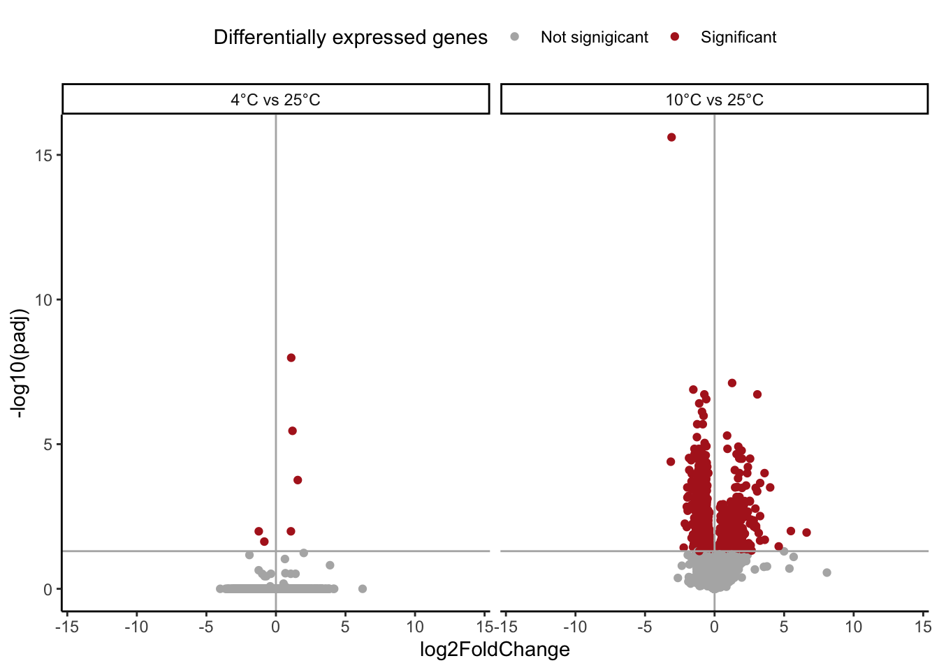
# Volcano Plots --
# Cold only
res %>%
filter(temp == "res_10" | temp == "res_04") %>%
mutate(temp = case_when(temp == "res_04" ~ "4°C vs 25°C",
temp == "res_10" ~ "10°C vs 25°C",
temp == "res_34" ~ "34°C vs 25°C",
temp == "res_37" ~ "37°C vs 25°C")) %>%
mutate(temp = factor(temp, levels = c("4°C vs 25°C",
"10°C vs 25°C",
"34°C vs 25°C",
"37°C vs 25°C"))) %>%
filter(!is.na(padj)) %>%
ggplot() +
geom_point(aes(x = log2FoldChange,
y = -log10(padj),
color = padj < 0.05)) +
geom_vline(xintercept = 0,
color = "grey70") +
geom_hline(yintercept = -log10(0.05),
color = "grey70") +
scale_color_manual(values = c("grey70",
"firebrick",
"grey80"),
name = "Differentially expressed genes",
label = c("Not signigicant", "Significant")) +
xlim(c(-14,14)) +
theme_classic() +
theme(legend.position = "top") +
facet_wrap(~ temp)
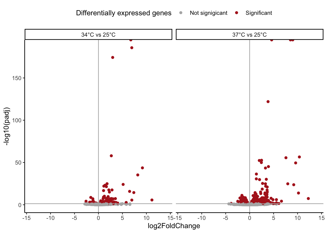
# Hot only
res %>%
  filter(temp == "res_34" | temp == "res_37") %>%
  mutate(temp = case_when(temp == "res_04" ~ "4°C vs 25°C",
                          temp == "res_10" ~ "10°C vs 25°C",
                          temp == "res_34" ~ "34°C vs 25°C",
                          temp == "res_37" ~ "37°C vs 25°C")) %>%
  mutate(temp = factor(temp, levels = c("4°C vs 25°C",
                                        "10°C vs 25°C",
                                        "34°C vs 25°C",
                                        "37°C vs 25°C"))) %>%
  filter(!is.na(padj)) %>%
  ggplot() +
  geom_point(aes(x = log2FoldChange,
                 y = -log10(padj),
                 color = padj < 0.05)) +
  geom_vline(xintercept = 0,
             color = "grey70") +
  geom_hline(yintercept = -log10(0.05),
             color = "grey70") +
  scale_color_manual(values = c("grey70",
                                "firebrick",
                                "grey80"),
                     name = "Differentially expressed genes",
                     label = c("Not signigicant", "Significant")) +
  xlim(c(-14,14)) +
  theme_classic() +
  theme(legend.position = "top") +
  facet_wrap(~ temp)
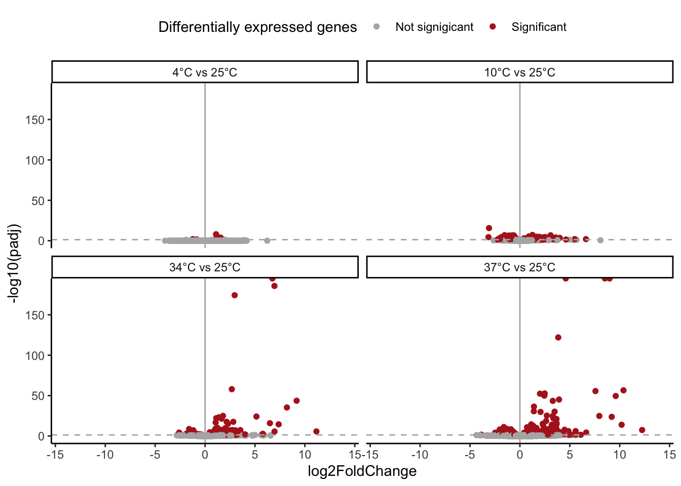
# All four comparisons
res %>%
  mutate(temp = case_when(temp == "res_04" ~ "4°C vs 25°C",
                          temp == "res_10" ~ "10°C vs 25°C",
                          temp == "res_34" ~ "34°C vs 25°C",
                          temp == "res_37" ~ "37°C vs 25°C")) %>%
  mutate(temp = factor(temp, levels = c("4°C vs 25°C",
                                        "10°C vs 25°C",
                                        "34°C vs 25°C",
                                        "37°C vs 25°C"))) %>%
  filter(!is.na(padj)) %>%
  ggplot() +
  geom_point(aes(x = log2FoldChange,
                 y = -log10(padj),
                 color = padj < 0.05)) +
  geom_vline(xintercept = 0,
             color = "grey70") +
  geom_hline(yintercept = -log10(0.05),
             color = "grey70",
             linetype = 2) +
  scale_color_manual(values = c("grey70",
                                "firebrick",
                                "grey80"),
                     name = "Differentially expressed genes",
                     label = c("Not signigicant", "Significant")) +
  xlim(c(-14,14)) +
  theme_classic() +
  theme(legend.position = "top") +
  facet_wrap(~ temp)
# Let's convert to gene symbol from FBgn
library(AnnotationDbi)
#
# Attaching package: 'AnnotationDbi'
# The following object is masked from 'package:MASS':
#
# select
# The following object is masked from 'package:dplyr':
#
# select
library(org.Dm.eg.db)
#
res$symbol <- mapIds(org.Dm.eg.db,
keys = res$FBgn,
column = "SYMBOL",
keytype = "FLYBASE",
multiVals = "first")
# 'select()' returned 1:1 mapping between keys and columns
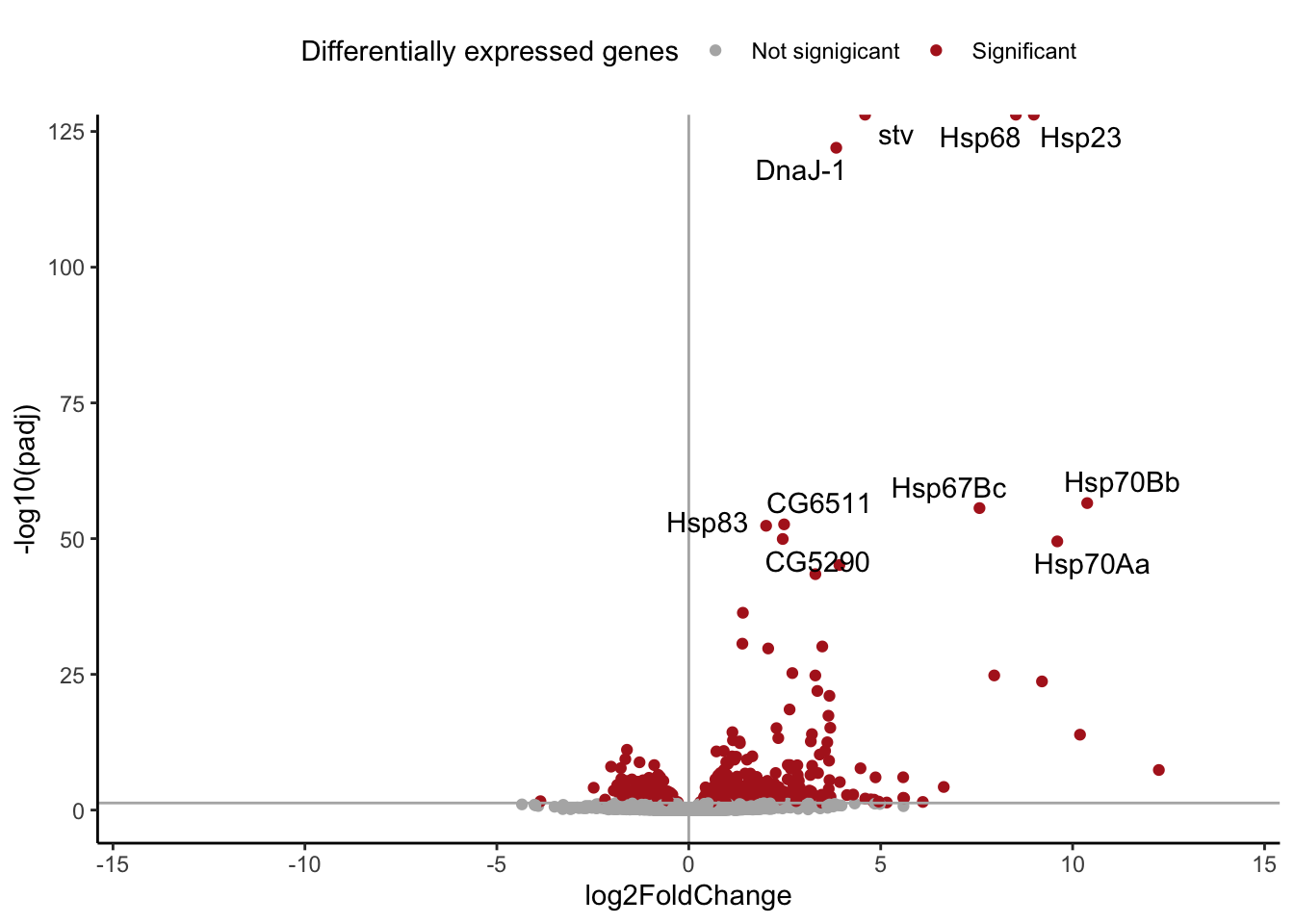
# Let's try and add symbols to the volcano plot
res %>%
filter(temp == "res_37") %>%
filter(!is.na(padj)) %>%
ggplot(aes(x = log2FoldChange,
y = -log10(padj))) +
geom_point(aes(color = padj < 0.05)) +
geom_vline(xintercept = 0,
color = "grey70") +
geom_hline(yintercept = -log10(0.05),
color = "grey70") +
geom_text_repel(data = res %>%
filter(temp == "res_37") %>%
arrange(padj) %>%
head(10),
aes(label = symbol)) +
scale_color_manual(values = c("grey70",
"firebrick",
"grey80"),
name = "Differentially expressed genes",
label = c("Not signigicant", "Significant")) +
xlim(c(-14,14)) +
theme_classic() +
theme(legend.position = "top")